Separate Excel List with Automatic Lines

When you create a table in Excel, you can use the built-in styles, to add bands of colour.

ConditionalFormatSections

The colour bands can make the table easier to read, because you can follow each line across, using the colour as a visual guide.

Separate the Days in the List

If you’re working with a list of tasks or orders, sorted by date, those coloured bands don’t help you see where each day’s data starts and ends.

To make it easy to separate the days, you can add conditional formatting to the table. We’ll add a line at the start of each date, to highlight those rows.

  • Select all the cells in the body of the Excel table. In this example, cell A2 is the active cell, and A2:F9 are selected.
  • On the Ribbon’s Home tab, click Conditional Formatting, then click New Rule

ConditionalFormatSections02

  • In the New Formatting Rule dialog box, click Use a Formula
  • In the formula box, enter this formula, which compares the values in cells A1 and A2. There is a $ before each A, because we need an absolute reference to column A.
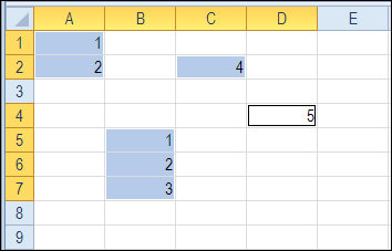
    • =$A2 <> $A1

ConditionalFormatSections05

  • Click the Format button
  • In the Format dialog box, click the Border tab
  • Select a border pattern and colour, to separate the dates. Unfortunately, you can’t select a thickness for the border line.
  • Click the top border in the preview window, and click OK

ConditionalFormatSections03

  • Click OK to close the New Formatting Rule dialog box.

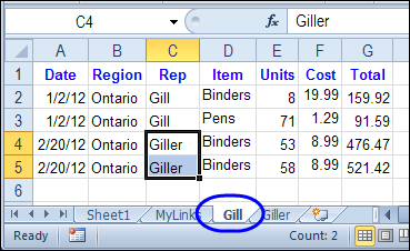
There will be a border at the start of each date in the table, and you’ll see at a glance where the dates start and stop.

ConditionalFormatSections04

More Conditional Formatting Examples

You’ll find many more conditional formatting examples and tutorials on the Contextures website.

Watch the Excel Video Tutorial

To see the steps for adding lines between the dates, you can watch this short Excel video tutorial.

___________

Data Validation Documenter

If your Excel file has many cells with data validation, it can be difficult to remember what restrictions you’ve put on the worksheet cells.

These tips show you how to find the data validation cells, and create a list of what rules are on the cells.

Select All the Data Validation Cells

If you just want to see where all the data validation cells are, you can use the command on the Excel Ribbon.

  1. On the Excel Ribbon, click the Home tab
  2. In the Editing Group, click Find & Select
  3. Click Data Validation
Go To Data Validation

This command selects all the data validation cells on the active sheet.

datavaldocument02

Select Specific Data Validation Cells

If you have different data validation rules on the active sheet, you can select only the cells that have the same validation as the active cell.

In the example shown below, cell D6 is active, and it has a data validation drop down list, based on the named range — DaysList.

datavaldocument05

To select any other cells on the active sheet with the same validation rule:

  1. With cell D6 active, click the Excel Ribbon’s Home tab
  2. In the Editing Group, click Find & Select
  3. Click Go To Special
  4. In the Go To Special dialog box, click Data Validation
  5. Click Same, then click OK

datavaldocument03

In the screen shot below, cell D7 was also selected, because it has the same validation rule as cell D6.

However, cell D4 was not selected, because its drop down list is not based on the same named range.

datavaldocument04

Create a List of Data Validation Cells

The Go To Special commands let you select the data validation cells, but they don’t show you the data validation rules. You would have to check each cell, or group of cells, to see its data validation rules.

datavaldocument06

If you want the details on each data validation cell for the active sheet, you can use a macro that compiles a list of details.

On the Contextures website, there is a Data Validation Documenter page. On that page, you’ll find sample code that creates a list of data validation details for the active worksheet.

In the sample file, there are two macros –

  1. DataValDocumenter and
  2. DataValDocumenterSheet

Both macros create a list of the data validation cells on the active worksheet, with the following details:

  1. Cell address
  2. Data validation type
  3. Data validation formula.

The DataValDocument macro creates the list in a text file, named Test.txt, in Excel’s default file location.

datavaldocument08

To see your default location, click the Excel Ribbon’s File tab, then click Options, and click the Save category. (in Excel 2003, choose Tools | Options, General tab)

datavaldocument07

In the DataValDocumenterSheet macro, a new worksheet is inserted at the front of the workbook, with a list of the data validation on the active sheet.

datavaldocument09

Download the Data Validation Documenter

You can download the data validation documenter file from the Contextures website.

To run one of the macros:

  1. Click the Ribbon’s View tab, then click Macros (In Excel 2003, choose Tools>Macro>Macros)
  2. Select DataValDocumenter or DataValDocumenterSheet
  3. Click the Run button

_______________________

Select Actual Used Range in Excel Sheet

It’s easy to select the current range in Excel – just press Ctrl + A. That shortcut selects all the cells in the block that surround the active cell. The selection stops at the first blank row and blank column. But how can you select actual used range in Excel sheet?

Continue reading “Select Actual Used Range in Excel Sheet”

Keep Track of Time in Excel

If you’re working on a project, you might need to keep track of time in Excel, so you can tell a client how much time you’ve spent on their project, and get paid for your work. Or, use the time data to see how much of your day is spent on productive tasks, and how much is spent Googling and tweeting.
Continue reading “Keep Track of Time in Excel”

Filter Excel Data Onto Multiple Sheets

There is a sample Excel file on my Contextures website that has a list of orders, and sales rep names.

It has a macro to filter Excel data onto multiple sheets. You can click a button, and a sheet is created for each sales rep, with that person’s orders.

Continue reading “Filter Excel Data Onto Multiple Sheets”

Excel Formulas Not Calculating

What happens when good Excel formulas go bad? A workbook of mine that worked fine for several years, when using Excel 2003, suddenly refused to update all the formulas, after a switch to Excel 2010. Even more mysterious, the calculations worked fine on some machines, but not others. Why are Excel formulas not calculating on some computers?

Hint: It wasn’t one of the obvious solutions.

Continue reading “Excel Formulas Not Calculating”

Efficient Navigation in Excel Workbooks

When I saw the signs in this shop window, I laughed, and snapped this picture.

Shop window with sign pointing to door handle

How confused are your customers, if you need a sign that says, “This is the door”, and another sign that points to the door handle?

Design Flaws

Later, I realized that it’s not a customer problem – it’s a design problem. A substantial number of people had trouble finding the handle, which looks more like a box. And I don’t remember exactly what the front of the store looked like, but the door must have been hard to identify too.

How about your Excel workbooks – are they easy to understand and navigate? I’ll admit that some of the spreadsheets I’ve built might have similar navigation problems. I’ve added arrows that point to data entry cells, and text boxes with user instructions. Not much different from that door!

Navigating a Workbook

What can you do to make Excel navigation easier?

In a large workbook, a menu sheet, with links to other sheets, is helpful. And all the other sheets should have a link back to that menu sheet.

hyperlinkclick

On a large worksheet, you can add a menu at the top of the sheet, linking to the sections below.

tableofcontentssheet05

If users can enter data on some sheets, group all the data entry cells in one area, and use colour coding, to make the cells easy to identify.

dataentry15

Worksheet Design Resources

Where do you get your worksheet design ideas? From your own experiments? From sample workbooks that you’ve found online? Somewhere else?

Even though it’s focused on web site design, rather than spreadsheets, I found plenty to think about in Don’t Make Me Think, by Steve Krug.

There are good tips in Professional Excel Development, by Rob Bovey, et al.

What books or other resources would you recommend?

________

Show Specific Info in Tabbed Excel UserForm

To show instructions to users in your Excel files, you can addworksheet  comments or text boxes with notes.

text boxes with notes

Excel UserForm With Help Info

Another option is to put the notes in an Excel Userform, and add a Help button on each worksheet.

The button can open the Help form to a specific page, and show the relevant Help information.

UserFormHelp02

Worksheet Help Buttons

This screen shot shows the UserForm Help page that open when you click a Help button on a worksheet.

In this example, the PivotSales sheet is active in the workbook, and its Help button opens the Pivot page in the UserForm’s MultiPage control.

UserForm opens at specific tab

Download the Sample File

You can download the sample file, and see the written steps, on the UserForm MultiPage Help page, on my Contextures website.

Watch the Video

To see the steps for creating the UserForm and Help buttons, you can watch this Excel video tutorial.

__________

Excel AutoFilter by Typing Criteria

Someone emailed me for help with an Excel AutoFilter last week. He wanted to type the criteria onto a worksheet, and have the filtered results shown automatically.

There are some built-in options for filtering by text, and keep reading to see a worksheet version that Roger Govier designed.

AutoFilter Search in Excel 2010

There is a new feature in Excel 2010 that provides easy searching, though not on the worksheet. You can see an example here, for the Excel 2010 AutoFilter search feature.

image

AutoFilter Search in Earlier Versions

In earlier versions of Excel, you can filter for text, but it’s a bit more work. In Excel 2007 you can use a text filter, which opens the Custom AutoFilter dialog box

image

In Excel 2003, use the Custom option on the AutoFilter drop down.

image

Roger Govier’s FastFilter

If you’d like to enter the AutoFilter criteria on the worksheet, instead of a search box or dialog box, you can use Roger Govier’s FastFilter sample Excel file.

He has set up a table on the worksheet, with an empty row above the table. In that row, you can type one or more criteria, and when you press the Enter key, the table is automatically filtered.

For a simple filter, type an exact match for a value, and press Enter. In the screen shot below, the table is showing only the items from category 2.

fastfilter01

You can also use operators, and in the next screen shot I’ve added a “>20” criterion in the Unit Price column.

fastfilter02

Use WildCard Characters

If you’re trying to find a specific string of characters in a column, you can use the * and ? wildcard characters. In the next screen shot, I used *b* in the product name column, to find any products that have a “b” somewhere in the name.

fastfilter03

Use Multiple Criteria in a Column

You can use special characters for OR (^^) and AND (^), to combine multiple criteria in a single heading cell. In the Category ID column, I used the ^^ characters to find category 2 OR 4. In the Unit Price column, the ^ character limits the price to >20 AND <35.

fastfilter04

Remove the Criteria

To clear the filter from a column, just click on the criteria cell, and press the Delete key on your keyboard. If you want to clear all the filters, select all the criteria cells, and press Delete.

Download the Sample File

To download the sample file, you can visit Roger’s Sample Files page on the Contextures website. In the Filters section, look for FL0001 – Fast Filter. There is a download link for the FastFilter zipped file.

The file is in Excel 2003 format, and will work in later versions too. After you open the file, enable macros, so you can test the automatic filter feature.

____________