
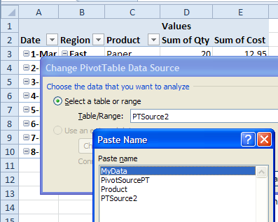
If you want to change the data source for a single Excel Pivot Table, you can use a command on the Ribbon. If you want to change data source for all pivot tables in a workbook, you can use a macro, instead of making the changes manually.
How to Show Excel Preview Picture When Opening Files
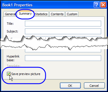
When you’re opening files in Excel, you can see the file Details, or the icons, or select another way to look at the list, such as Preview.
That Preview option sounds promising, but instead of a picture of the file’s contents, you usually see this message instead – Preview Not Available.
And that’s not much help. Here’s how to show Excel preview picture when opening files
Continue reading “How to Show Excel Preview Picture When Opening Files”
Change Pivot Table Filter All Sheets or Active Sheet
In Excel 2010, you can use Slicers to change the filters in several pivot tables, with a single click.
If you don’t have Excel 2010, or don’t want to use Slicers, you can use programming to change multiple pivot table filters with a single click.
Yes, it’s more work than adding a Slicer, but better than manually changing all those pivot tables!
Change All Pivot Tables
Last December, I described how to add code to your workbook, so if you changed one pivot table filter, all the other pivot tables in the workbook would change too.
Click here to read that article, and the comments: Change All Pivot Tables With One Selection
In those comments, people asked how to modify the code, so only the pivot tables on the active sheet were affected, or only a specific field was changed.
In response to those comments, I’ve created a new version of the sample file.
Change All Pivot Tables or Active Sheet Only
The latest sample file for changing pivot table fields has 3 variations on the “Change All Page Fields” code.
It also changes the “Multiple Item Selection” settings to match changed page fields (Excel 2007 and Excel 2010 only).
The three variations are:
- Change any page field in a pivot table, and all matching page fields, on all sheets, are changed.
- Change any page field in a pivot table, and all matching page fields, on the active sheet only, are changed.
- Change a specific page field in a pivot table, and that page field, on the active sheet only, is changed.
Download the Sample File
To see the code, and try the variations, you can download the sample file from the Contextures website. The file will work in Excel 2007 or Excel 2010, if you enable macros.
PT0027 – Change All Page Fields – All Sheets or Active Sheet
You can also download the other sample files, showing how to change a specific field, or all fields, in the workbook’s pivot tables.
PT0008 – Change Multiple Page Fields
PT0015 – Change Multiple Different Page Fields
PT0016 – Change Page Fields With Cell Dropdown
PT0021 – Change All Page Fields
PT0025 – Change All Page Fields with Multiple Selection Settings
______________
Show Excel Chart or Data in Dashboard With No Macros
In this Excel dashboard example, you can select “Chart” or “Chart Data” from a drop down list. Magically, with no macros in the workbook, the selected item appears on the worksheet.

With this technique, you can store your data and chart on a hidden sheet in the workbook, where no one can mess with the numbers. (Not that anyone would!)
Continue reading “Show Excel Chart or Data in Dashboard With No Macros”
Copy PivotTable Style
Yesterday, i created a custom PivotTable Style for a customer, to make it easy to format multiple pivot tables, using their corporate colour scheme.
PivotTable Styles are available in Excel 2010 and Excel 2007, and if you don’t like the existing styles, you can create your own custom styles, and apply those to any pivot table.
Copy Custom PivotTable Styles
Unfortunately, there’s no built in way to copy a custom PivotTable style from one workbook to another.
A while ago, I made this video, to show you a workaround for copying your favourite styles to a different workbook.
Remove Existing Formatting
If you’re applying a built-in or a custom style to a pivot table, you might need to remove any manually applied formatting first.
- Instead of clicking on the PivotTable Style icon, right-click on it.
- Then, click Apply and Clear Formatting
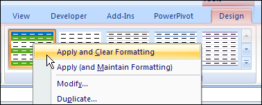
You might need to tidy up the pivot table after you apply the new style, but with Custom Styles you can quickly format your pivot tables, so they have a consistent appearance.
______________________
Data Entry Shortcuts for Dates and Numbers
Are you working hard this week? Instead of doing all the work yourself, let Excel do some of the data entry for you. These quick tips show you how to enter a date or number series, with a minimum of effort.
Enter a Series of Numbers
With this shortcut, you can quickly create a series of numbers on an Excel worksheet, such as a series of even numbers or odd numbers.
- To start the series, type the first two numbers in adjacent cells.
- Then, drag the Fill Handle to continue the series on the worksheet, as far as you need it to go.
This Excel Quick Tips video shows you how to fill the series, and there are many more Excel Data Entry tips on the Contextures web site.
Enter a Series of Dates
With the next shortcut, you can create a series of dates on an Excel worksheet, incremented from your starting date.
- To start the series, type the first date in a cell.
- Then, drag the Fill Handle to continue the date series on the worksheet, as far as you need it to go.
This Excel Quick Tips video shows you how to fill the date series.
Create Excel List of Dates by Week
With the final shortcut, you can create a series of dates, by week, on an Excel worksheet, incremented from your starting date.
- To start the series, type the first date in a cell.
- Then, press the right mouse button while you drag the Fill Handle to continue the weekly date series on the worksheet, as far as you need it to go.
- Release the mouse button and click Series in the popup menu.
- Type a 7 as the Step value, and click OK.
This Excel Quick Tips video shows you how to fill the date series.
__________________
Create an Excel UserForm
This week, I’ve been working on a client’s Excel file, and we’re using a UserForm for data entry, instead of worksheet cells.
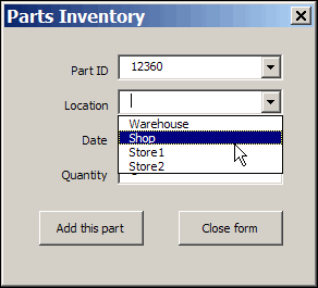
Data Entry and Storage
Data can be entered in the UserForm, and stored in a worksheet, when the form is closed.
The UserForm could open automatically when the file opens, or put a button on the worksheet, and click that to open the form.
On the Contextures website, you can find instructions and sample workbooks, for creating a simple UserForm, or a UserForm with drop down lists.
Watch the Excel UserForm Videos
To see the steps for creating an Excel UserForm, you can watch this 3-part Excel Video Tutorial series.
You’ll see how to add a UserForm to your Excel file, then put text boxes and buttons on the form.
Demo – Excel UserForm for Data Entry Demo
Creating a UserForm – Part 1
In part 1, you’ll see how to create a blank Userform. Then you’ll name the UserForm, and next you’ll add text boxes and labels.
Users will be able to type data into the text boxes. Labels are added beside the text boxes, to describe what users should enter into the text box
Creating a UserForm – Part 2
In Part 2, you’ll learn how to add buttons and a title on the UserForm.
With buttons on the UserForm, a user can click to make something happen.
For example, click a button after entering data in the text boxes, when you’re ready to move the data to the worksheet storage area
Creating a UserForm – Part 3
In Part 3, you’ll learn how to add VBA code to the controls, and you’ll see how to test the UserForm.
The VBA code runs when a specific event occurs, such as clicking a button, or entering a combo box. In this example, the user will click a button, and the VBA code will move the data to the worksheet storage area
Creating a UserForm – Part 4
In Part 4, you’ll see the code that adds the items to the combo boxes.
____________
Excel VLOOKUP Week Sharks
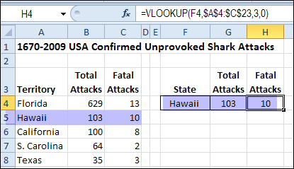
It’s Excel VLOOKUP week, as announced on the Microsoft Excel team’s website. Chandoo had a VLOOKUP Week in November 2010, so I guess it only comes around every 18 months or so – don’t miss it.
Drill to Detail With Excel Slicer Filters
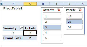
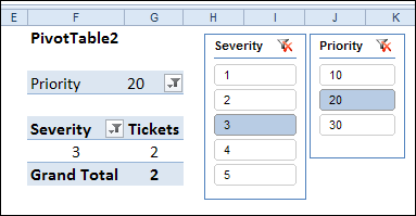
With Slicers in Excel 2010, you can easily filter several pivot tables with a single click. In the screen shot below, the Slicers are filtering the Severity and Priority fields in the pivot table.
However, there is a problem with Drill to Detail with Excel Slicer Filters, in some version.
Continue reading “Drill to Detail With Excel Slicer Filters”
How to Spot the Old Excel File
 I’m going cross-eyed this week, working with an Excel workbook that is full of rating tables.
Last week, I converted the rating manual from PDF format to an Excel file.
Setting Up Formulas
Now I’m setting up the formulas, to pull the correct rating data for the selected criteria.
Many of the tables have changed in structure from the previous version, so there are lots of adjustments required in the workbook.
While I work on the new version of the Excel file, occasionally I need to check the previous version, to see how things were set up there.
Don’t Edit the Wrong File
The danger in having multiple copies of an Excel file open is that you might accidentally make changes to the old file, instead of the new one. Of course, that’s never happened to me, but a close friend had that problem once. 😉
But seriously, as you flip between files, and click on different sheets in those files, it is easy to forget where you are.
You change a few formulas, add items to a list, and save your work. And that’s when you realize the you spent time editing the old file. Sigh.
Spot the Old File
Today, while working with the old file and the new one, I wanted a foolproof way to know which file was active. First, I thought about adding fill colour to the first few rows of each worksheet in the old file.
That wouldn’t work too well though, because there was colour coding in some of those cells already.
Then it dawned on me – I could colour all the sheet tabs in the old file. The file didn’t use tab colouring, so that would make it easy to tell the files apart.
Change Tab Colour
To add the tab colour in the old Excel file, I did the following:
- Right-click on any sheet tab, and click Select All Sheets
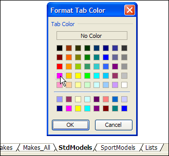
- Right-click on one of the tabs, and click Tab Color.
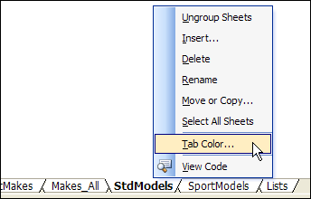
- Click on the colour that you’d like to use for your old file – I picked bright pink – then click OK.
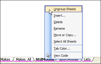
- Right-click on one of the sheet tabs, and click Ungroup Sheets.
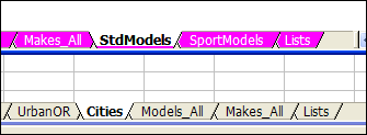
Now, it’s certainly easy to see which file is the old one. Don’t make any changes in the file with the pink tabs!
__________