
In a pivot table, you might have a few row labels or column labels that contain the text “(blank)”. This happens if data is missing in the source data. For example, in the source data, there might be a few sales orders that don’t have a Store number entered.
Why Excel Ignores Spelling Errors-Fix
Why is Excel ignoring your spelling mistakes, like the one shown in the screen shot below? That’s not how you spell Capital!
However, the Excel message cheerfully says, “The spelling check is complete for the entire sheet.”

Upper Case Entries
If you use upper case for headings in Excel, or anywhere else on your worksheet, any spelling errors in them might go uncorrected.
That’s what happened with “CAPITEL “, in the example shown above.
To make sure that any UPPER CASE text entries are included in a spelling check, you can change an option in Excel, as shown below.
Change the Spelling option in Excel 2007
- To get started, click the Office button, at the top left of the Excel window.
- Next, click the Excel Options button
- In the Excel Options window, at the left, click the Proofing category
- at the right, scroll down to the section, When correcting spelling in Microsoft Office programs…
- In that section, remove the check mark from ‘Ignore words in UPPERCASE’
- Finally, click the OK button, to close the Options window
Change the Spelling option in Excel 2003
If you’re using Excel 2003, follow these steps to change the spelling setting:
- First, click the Tools menu, and then click Options
- Next, click the Spelling tab
- Remove the check mark from ‘Ignore words in UPPERCASE’ and then click OK
__________________
Macro Creates Excel Workbooks For Entire Year
Roger Govier has created an Excel file with a macro that will set up a year’s worth of workbooks for you, at the click of a button.
It might not be the ideal workbook setup, but some people need to set these up, and this macro will certainly make the task easier.
Macro Creates Monthly Workbooks
This macro will create a series of 12 workbooks in the same folder as this workbook is stored.
You’ll be prompted to enter the year number at the beginning of the macro.
Each new workbook will be named with month and year e.g. Jan 2009.xls through Dec 2009.xls
Daily Sheets Each Month
Within each workbook, there will be a sheet for each day of the month.
There’s an option to display the numbers as ordinals, so if you click Yes for that, the sheet names would be Jan 1st, Jan 2nd and so on.

Get the Sample File
To download the Excel file, and to see the written steps, you can go to the Create Workbooks and Worksheets page on my Contextures site.
The zipped file contains a macro, so be sure to unblock them in Windows Explorer, before you open them.
After you open the file, enable macros, when the security message appears.
_________________________
Free Excel Conference Microsoft London April 2009
The UK Excel User Group is holding a free conference at Microsoft London in April 2009. It’s a bit too far for me, but if you can make it, I highly recommend that you register.
You’ll learn new things, meet some terrific people, and spend a couple of days discussing Excel. What could possibly be better than that?
The agenda includes sessions on charts, pivot tables, functions, names and many other topics. Even if you’re familiar with some of the topics, you’ll benefit from attending.
Excel Expert Presenters
The presenters are a very smart and creative bunch, and they’ll almost certainly show you a few tips and techniques that you haven’t tried before.
The Q&A sessions will be an excellent opportunity to discuss any Excel problems that you’ve encountered, and get solutions or suggestions from the presenters and other attendees.
When and Where
- Date: April 1-2, 2009
- Location: Microsoft London (Cardinal Place)
- 100 Victoria Street
- London SW1E 5JL
- Tel: 0870 60 10 100
The agenda for the two days is outlined at the Excel User Group site and there’s also a Word document with conference details that you can download.
To book for either or both days, send an email to [email protected]
Tell them that Debra sent you, and you’ll get a 25% discount on the free admission! You can use Excel to figure out how much that is! 😉
_____________________________
Show Word Comments in Balloons
I’m reviewing Word files and inserting comments for the author. I’d like to see show Word comments in balloons along the sidebar, but Word won’t cooperate, and shows them in a Reviewing Pane, at the bottom of the window. Here’s how to fix the problem
Count Blank Cells in Pivot Table Source Data
Sometimes there are blank cells in a pivot table’s source data. If you try to count blank cells in Pivot Table source data fields, you might run into a problem.
Here are the steps to follow, to show the count of blanks.
Continue reading “Count Blank Cells in Pivot Table Source Data”
Make Excel Box and Whisker Chart-Box Plot Chart
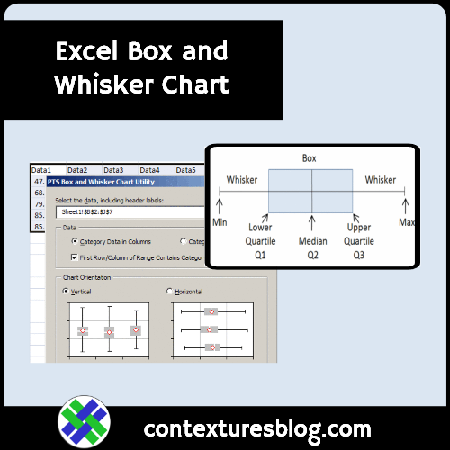
What the heck is a box and whisker chart, and why would you need one? Well, I’m not a statistician, but here’s my overview.
Continue reading “Make Excel Box and Whisker Chart-Box Plot Chart”
Convert Excel Numbers to Roman Numerals
Recently, I read a business article that said you should “become a Roman” to succeed in business. By that, the author meant, “be disciplined and willing to keep fighting”.
Excel ROMAN Function
Maybe that’s why we have the Excel ROMAN function! It will quickly convert a worksheet number into Roman numerals.
That frees up our time, so we can “keep fighting” to fix other problems in our Excel files.
In the sections below, I’ll show you how the ROMAN function works. And I found a couple of fun facts about ROMAN, that might impress your friends and co-workers. (Or not!)
Excel ROMAN Function Syntax
Here are the two arguments in the ROMAN function:
- number: an Arabic number, between 0 and 3999, that you want to convert to Roman numerals.
- form: (optional) the type of conciseness that you want to display.
Tip: Read about the standard Roman numeral format, and other forms, on the Wikipedia Roman Numerals page.
1. Number Argument
For the number argument, you can type the number into the formula, or refer to a cell that contains a number between zero and 3999
At first, I incorrectly assumed that the 3999 was an Excel limit, but that’s not the reason. Instead, I learned that 3999 is a Roman numeral limit.
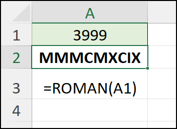
- The largest number that can be represented in standard Roman numeral form is 3999
- That number is written as MMMCMXCIX in Roman numerals
2. Form Argument
On those rare occasions when I use the ROMAN function, I always omit the second argument, form.
- If you omit the 2nd argument, or use TRUE or zero, the result is a classic Roman numeral, that you probably learned in school.
Form Argument Omitted
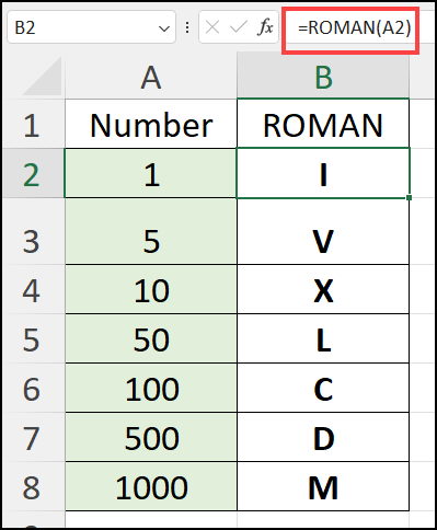
In the screen shot below, I entered 7 numbers in column A, and the ROMAN function, with the 2nd argument omitted, in column B.
NOTE: Those are the only 7 characters used to create any Roman numeral:
- I, V, X, L, C, D, M
Levels of Conciseness
For the Form argument, you can also use numbers between 1 and 4, as well as FALSE.
- Numbers 1 to 4 create more concise versions of the Roman numeral.
- The higher the number, the greater the level of conciseness.
- FALSE is Simplified form, the same as number 4
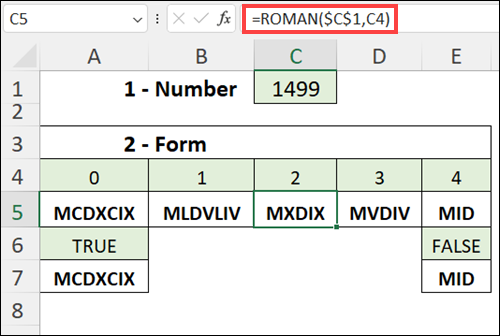
Some numbers will show different Roman numeral, depending on the form argument. Other numbers will have the same Roman numeral for all forms.
- For example, in the screen shot below, number 1499 has a different Roman numeral for each form.
- The number 115 (not shown) has the same result for all forms
Also, the results below show that
- TRUE is the same as zero
- FALSE is the same as 4
Excel Function Tutorials
These tutorials, on my Contextures site, show how to use some of the most popular Excel functions.
To see full list of Excel functions, visit the Excel Functions List page.
1 — How to Sum Cells – Start with the SUM function, then try SUMIFS and more!
2 — Count All or Specific Cells – Do a simple count, or count based on criteria
3 — How to Do a VLOOKUP – Find a lookup item in a table, such price for specific product
4 — Lookup With Criteria – Use formulas to get values from a lookup table, based on multiple criteria
5 — Combine Text & Numbers – Use formulas to combine values text and numbers from different cells
__________________________
Clearing Out the Deadwood
Last weekend a friend, aka Chauncey, who has some gardening knowledge, came over to help trim the trees and shrubs in the back yard.
About an hour later, much of the lawn was covered with branches, twigs and leaves.
It took another couple of hours to stuff everything into yard waste bags, and bundle the big pieces.
This week it’ll be taken to the city recycling centre, where it will be turned into compost or mulch.

It was way more work than I expected, but the catalpa tree, which was overgrown, now looks much better.
Chauncey claims it will flourish in the spring, without all the extra branches.

Clear the Office Too
When I got back to my office, I realized that I should do the same thing there.
So, next weekend I’ll clear out more of the deadwood in the office — old paper files, computer programs that I’m no longer using, RSS feeds that I never read, links to time-wasting web sites, and old email with large attachments that I don’t need.
All that stuff is slowing me and my computer down, and a few hours of work should make other things go faster when I’m finished the cleanup. I hope!
__________________________________
Enter the Time in a Notepad File
I like to use Notepad to make notes as I work. In July, I described how I type .LOG at the top of the Notepad file, so the date and time are automatically entered when the file opens.
That’s a handy feature, but I wanted to timestamp the files as I was working to, to record my start and stop times. There are date and time shortcuts in Excel and Access, but unfortunately those shortcuts don’t work in Notepad.
I obviously hadn’t looked too hard, because today I found the shortcut that I’ve been looking for — listed right there on the Edit menu in Notepad.
Now, if I want to insert the date and time, I press the F5 key, and it’s automatically entered for me.

========================