
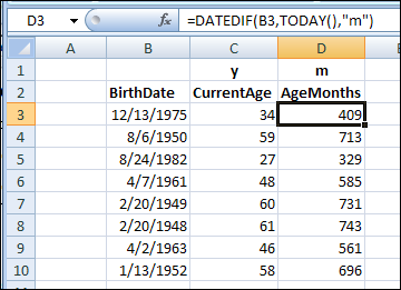
Can you remember how old you are? Or are you like me, and have to ask, “What year is it?” and then subtract your birth year? Or do you like calculating ages in Excel — let it do the arithmetic for you!
Excel Movies Database Filter Macro
The Oscar nominations will be announced next Tuesday, February 2nd (oh, Groundhog Day, that was a good movie).
In honour of the occasion, I’ve updated my Excel Movie Database sample file.
Excel Movie Database
I included some movies from the Top 250 Movies list at the IMDb website. You can add movies from your DVD collection, or your Netflix list.
Then use the selection boxes to see movies from a specific category, and/or featuring your favourite actor.
In the previous version, you could only choose Category OR Actor, and now you can choose one or both. (Exciting, I know!)
Or, clear both criteria cells, to see all the movies.

Download the Sample File
You can download the Excel movies database file from the Contextures website. It’s in Excel 2003 format, and zipped.
The file contains macros, so you’ll have to enable those to make the file work.
The Perfect Computer
I couldn’t find any movies about Excel, to add to the Excel movies database, but computers play a leading role in several movies. You might remember HAL 9000, from “2001: A Space Odyssey”.
HAL: Let me put it this way, Mr. Amor. The 9000 series is the most reliable computer ever made. No 9000 computer has ever made a mistake or distorted information. We are all, by any practical definition of the words, foolproof and incapable of error.
Yes, that was the dream, way back in 1968, when they made “2001: A Space Odyssey”. Over 40 years later, we haven’t even come close to achieving that goal! Well, maybe it’s not the computers’ fault – the users might be part of the problem.
Random Draw Sinner
Congratulations to Alex Kerin, whose name I selected in the random draw for the Excelerator Quiz giveaway. Here’s his name at the top of the list, after I used the RAND function, and sorted the Rand column in ascending order.

Alex’s prize is a 23″ monitor, plus a keyboard and mouse, courtesy of the PowerPivot team. Thanks to everyone who participated, and to the PowerPivot team, and Megan at Ignite Social Media, who organized the giveaway.
__________
Excel AutoFilter Shows Filter Mode
It’s Price Book publishing week for one of my clients, and we’ve been making lists, and checking them twice. Or 3 or 4 times, or more!
When comparing the new prices to the previous prices, an Excel AutoFilter comes in handy. You can select the same product or model in each workbook, and easily compare item details.
Yes, the widget prices went up a bit this year, so that’s why the assembled parts cost a bit more.
There are written steps and a video below, that show how to use the AutoFilter feature, and workarounds for a problem
Record Count in the Status Bar
Sometimes when you select records with an AutoFilter, the record count appears in the Status Bar, at the bottom left. In this example, I was working with a small table, with 50 records, and only one column had a formula.
I selected File Folder in the Product column, and the Status Bar showed that 3 of the 50 records contained that product. So far, so good.

Status Bar Shows Filter Mode
Then I added another record to the table, and selected a different product from the AutoFilter drop down list. This time the Status Bar showed the rather unhelpful message, “Filter Mode”, instead of the record count.

Excel 2007 seems to handle this better, but in Excel 2003, and earlier versions, you might see “Filter Mode” if there are more than 50 formulas in the list.
When you apply an AutoFilter, the formula recalculate. If there are lots of formulas to calculate, Excel shows a “Calculating %” message in the Status Bar, so you’ll have something to entertain you while you wait.
Unfortunately, the “Calculating %” message interferes with the record count message in the Status Bar. If the record count message is interrupted, it shows the “Filter Mode” message instead.
You can’t change this behaviour, but there are a couple of workarounds that you can use to find the record count.
Use AutoCalc Instead
If the Status Bar shows “Filter Mode”, you can get the record count from the AutoCalc feature instead.
- Right-click on the Status Bar
- In the pop-up menu, click Count Nums
- Click on the column heading for a column that contains numbers (and no blank cells within the list)
You’ll see the count of visible numbers in the AutoCalc area of the Status Bar.

Use the SUBTOTAL Function
If you’d rather have the record count show up automatically, you can use the SUBTOTAL function. It ignores the filtered rows, and calculates based on the visible rows only.
For example, with numbers in column D, this formula, with 2 as the first argument, will calculate the COUNT of visible numbers:
=SUBTOTAL(2,D:D)

If you want to count items in a column that contains text, use 3 as the first argument, and subtract 1 from the result, to account for the heading cell.
=SUBTOTAL(3,B:B)-1
Watch the Excel AutoFilter Video
In this very short video you can see my Excel AutoFilter experiment, and watch the Filter Mode message appear in the Status Bar.
There are no ruggedly handsome math teachers in this video, but it’s fun-filled and action-packed!
There are more Excel AutoFilter Tips on my Contextures website.
___________
Excel Codes Change to Scientific Notation
Let’s call this installment, “The Mysterious Case of the Vanishing Parts.” (Read carefully — that’s paRts, not paNts.)
Strange Formatting
Last Friday, I was working on a client’s Excel file, revising some VBA code.
The code splits a list of manufacturing parts into multiple columns, strips a couple of characters off the front of the part name, and copies the results to another column.
What Happened?
It seemed to be going well, until I got an email from my client, saying that some of the part numbers looked funny.
He included a screenshot, and indeed, those part numbers did look odd. Here’s an example, using some dummy data.

Scientific Notation Formatting
“Aha!” I thought. (Yes, I actually talk to myself like that. 😉 )
Those parts were all numbers, so Excel just formatted them as Scientific Notation.
I could simply format the column as General at the end of the macro, to make them look right.
Unfortunately, it wasn’t that simple. When I clicked on one of the affected cells, the formula bar showed 220 as the actual part number.
So, if I changed the formatting to General, 220 is the part number that would be copied to other cells, later in the macro.
That would cause problems, because all the codes should have two digits, then a letter, and then numbers

Why Part Number Was Changed
After a bit more investigation, I found that the original part number wasn’t 220, it was 22E1.
Close, but manufacturing might be adversely affected if Excel starts making up new part numbers!
Because the original part number (22E1) started with numbers, followed by the letter E, then another number, Excel interpreted it as a number in Scientific Notation.
It converted that number to Excel’s style of Scientific Notation (exponential) formatting – 2.20E+02.
I’m sure Excel was trying to help, but that creates problems, just as it does when Excel changes 6-10 to a date for you, without asking.
The workaround to this unsolicited help is to force the data to be recognized as text, as Microsoft explains in its article:
Text or number converted to unintended number format in Excel.
Fixing the Problem
In my client’s macro, instead of formatting the parts column after copying the part names, I added an apostrophe at the start of each part name.
The apostrophe doesn’t show on the worksheet, but it tells Excel that the cell contents are text.
That solution left the “E” parts in their original format, and the problem was solved.
VBA Code Revision
Here’s the formula that is added in the VBA code:
.Range(“D2?).Formula = “=IF($A2<>$A1,””‘”” & $U2,””””)”

Scientific Notation Explained
If you’d like to know how scientific notation works, in fairly simple terms, you can read this article: Scientific Notation
And for an even shorter and simpler description, here’s a short video in which a math teacher explains scientific notation.
And remember to do your homework!
_______________
Excelerators Giveaway for Excel Power Users
 Are you an Excel power user? Answer a few quick questions at the Excelerators Quiz site, and find out how you rate. You could even win a nice prize here at the Contextures blog!
The team at PowerPivot for Microsoft Excel 2010 created the Excelerators Quiz, and to make the challenge more exciting, they’re sponsoring a giveaway here on the Contextures blog (for USA residents only).
The blog giveaway prize has a total value of over $250, and will include a Dell ST2310 23 inch flat panel monitor, keyboard, and mouse. You’ll be even more powerful if you have those tools!
Enter the Giveaway
What does it take to be an Excel power user? What kind of quiz questions would you create? We’ll create our own Excel quiz here in the comments. Maybe it’ll be better than the Excelerators Quiz!
To enter the giveaway, after you take the Excelerators Quiz, come back here and add a comment. In your comment:
- Create your own unique question for the Excelerators Quiz.
- Make your question multiple choice, with the correct answer as one of the four options.
You can contribute more than one question, but only your first question will be entered in the giveaway draw.
The Giveaway Rules
- You must be a legal resident of the Unites States of America.
- To enter, submit an original Excelerators quiz question in the comments below, with the correct answer as one of the 4 multiple choice options
- The comment must be submitted before the deadline of 12:00 noon (Eastern Time) on Thursday, January 28th, 2010
- One entry per person – any additional entries will be deleted from the draw
- A random draw will select the winner from all valid entries.
- Winner will be notified by email, so please provide a valid email address. This will not be publicly visible, but will be shared with the contest organizers at Ignite Social Media, so they can contact the winner to arrange delivery.
The Alpha Geek Challenge
The PowerPivot team has also launched an Alpha Geek Challenge for more advanced excel geeks. Donald Farmer will host a PowerPivot competition in which the Grand Prize winner will receive an all-expenses paid trip to the 2010 Microsoft BI Conference in New Orleans, LA in June.
After you finish the Excelerators Quiz, and the giveaway contest here, see how you do in the Alpha Geek Challenge!
________
Excel OFFSET Function-Fish for Data
That’s my dad in the picture below, proudly holding the catch of the day. He tried to teach me how to fish, but without much success. (Worms…ewwww.)

Fishing with OFFSET Function
This week someone asked me to explain the Excel OFFSET function, saying “Please teach me to fish.” That’s when it struck me that using OFFSET is similar to fishing.
- When you’re fishing, you can dip into a pond with a bamboo pole and a small hook, or head out to sea, and cast a large net. Or you can fish the way we do in Canada, through a small hole in the ice, but that’s another story. (There’s a video at the end of this article.)
- With the Excel OFFSET function, you can pull data from a single cell nearby, or a large range of cells off in the distance.
The OFFSET function is useful when you want to make the data selection adjustable.
For example, if a February date is entered in cell A2, you can sum the February expense column. If a March date is entered, sum the March expenses instead.
Your Fishing Equipment
To make the OFFSET function work, you’ll tell it 3 things:
- The starting point
- Where to go from there
- How big a range to capture (optional)
The OFFSET syntax is: OFFSET(reference,rows,cols,height,width)
- The reference is the starting point.
- The rows and cols tell OFFSET where to go from the starting point. It can go up or down a specific number of rows, and left or right a specific number of columns.
- The height and width set the size of the range. It can be as small as 1 row and 1 column (a single cell) or much bigger.
For example, this OFFSET formula would return the January total, in cell B6:
=OFFSET(A1,5,1,1,1)
- The starting reference is cell A1.
- From there, it goes down 5 rows, and right one column, to cell B6.
- The selected range size is 1 row tall and 1 column wide.

Baiting the Hook
Instead of typing all the values in the formula, you can use one or more cell references, to make the OFFSET formula flexible. In this example, all the totals are in row 5, so that number won’t change.
However, the month number is typed in cell G1, so you could use that cell to set the number of columns to offset. Change the formula so G1 is the cols argument.
=OFFSET(A1,5,G1,1,1)

Now, if you change the month number to 3 in cell G1, the March total will be returned.
Casting the Net
Instead of pulling the result from a single cell, you could use OFFSET with the SUM function, to select a range with multiple cells, and calculate the total.
For example, this formula would calculate the total for the February expenses.
=SUM(OFFSET(A1,1,G1,4,1))
- The starting reference is cell A1.
- From there, it goes down 1 row, and right 2 columns, to cell C2.
- The selected range size is 4 rows tall and 1 column wide – C2:C5.

Other Fish to Fry
I like the OFFSET function, and use it to create dynamic ranges in some of my workbooks.
There are alternatives to using the Excel OFFSET function, such as the Excel INDEX Function.
There’s an interesting discussion of the merits of each function on Dick Kusleika’s Daily Dose of Excel Blog: New Year’s Resolution: No More Offset.
Ice Cold Fish
I’d rather stay inside and work on OFFSET formulas, but ice fishing is popular here in Canada. This video makes the sport look almost appealing.
_____________________
Athlete Height Weight Analysis Pivot Table
 Occasionally, a football game appears on the television at my house. I’m talking about real football, with burly men in tight pants, not that other kind of football, with wiry men in shorts.
This weekend, one of the games was between teams from Arizona and New Orleans. While admiring the strategies of the two teams, I noticed that the players whose numbers were in the 60s and 70s seemed heavier than the others.
Was that an optical illusion? Did their numbers, or some extra padding, make them seem bigger? Or were they really larger than the rest of the team?
Excel Weight Analysis
Excel can help you with burning questions such as these. From the NFL site, I copied the player roster for each team, and pasted it into Excel.
Unfortunately, the player heights were entered as feet-inches, e.g. 6-1, so that took a bit of fixing, because Excel helpfully changes numbers in that format to dates. A few players didn’t have numbers listed, so I changed those to zero.
Make a Pivot Table
After the player rosters were pasted into Excel, I created a pivot table from the data.
I put the player numbers into the pivot table Row area, Team name into the Column area, and Weight into the Values area, as Average.
Then I grouped the pivot table Player Numbers into 10s.

Average Weight in Pivot Table
As I suspected, the 60s and 70s are much heavier than their teammates. Only the 90s come anywhere close.

Maybe It’s Not the Number
Admittedly, I don’t know too much about how the player numbers are assigned. Maybe each position gets a specific number range and some positions need bigger players.
So, I created another pivot table, to check the average weight of players in each position, and see which numbers are assigned. A bit of conditional formatting was added, to highlight the different weight ranges.

And it does look like the Guards and Tackles are assigned numbers in the 60s and 70s. The lower numbers have lower weight players, and the 80s have a middle range.
BMI Status
Since we created a Body Mass Index formula a couple of weeks ago, I added that to the player stats too. Then a VLOOKUP formula pulled the BMI status from a lookup table, and a pivot table showed the number of players in each status (Normal, Overweight or Obese).
I’m sure their muscles put the players into different BMI categories than the rest of us, but there aren’t many guys in the Normal category.

Team Weights
Finally, I created a table to compare the player weights on each team. Overall, the Arizona team is a bit heavier. Maybe that slowed them down, and that’s why they lost the game.

Download the Workbook
If you’d like to do your own team weight analysis, you can download the sample workbook from my Contextures website. Go to the Excel Sample Data page, and scroll down to the Football Player section. The zipped file is in xlsx format, and does not contain any macros.
[Update – August 2022]: I’ve added 2022 player data to the workbook, for the same two football teams. Now there are 306 player records for you to analyze!
Anyway, the football season should be over soon, and the players can use the Excel Calorie Counter to get themselves in shape for next year. Only if they want to, of course – I’m certainly not going to mention weight loss to any of them!
_____________
Does Excel Drive You to Drink?
After a long day of dealing with Excel formulas, pivot tables, and hidden Ribbon commands, you might be ready for an evening cocktail. Or six!
Newspaper Study
I found a link to this Canadian drinking study in the Toronto paper today, and it looks like we’re a nation of teetotalers. Is your country the same?
Apparently most Canadians don’t work with Excel, or perhaps they vent their frustrations on the hockey or curling rink at the end of the day.

The Excel Drink Calculator
To spare you the agony of checking your results in a hard-to-read green pie chart, I created an Excel version of the online drink calculator.

Use the Drink Calculator
In cells C3 to C9, enter your estimated number of drinks per day.
- The SUM Function in cell C10 calculates your total for the week.
Then, select Men or Women from the drop down list in cell C12.
- The VLOOKUP formula in cell C15 will compare your results to the rest of the men or women in Canada.
Hmmm…more than 85% – that can’t be good.
Time to move, I think. 😉 What country would you recommend?
Download the Excel Drink Calculator
If you’re brave enough to test your own results, you can download the Excel Drink Calculator. It’s in Excel 2007 format, with no macros.
Please do not operate heavy machinery, or leave a comment, if you have been drinking.
______
Leno and Conan Excel Gantt Chart
Rumours say that the late night TV schedule on NBC will change. Jay Leno will leave his 10 PM spot, and return to 11:35 PM. How long will the revised Leno show be, and what effect will it have on the rest of the schedule?
I’ll bet the NBC programming executives have set up an Excel worksheet to test the possible scenarios, and they made a nice Gantt chart to show the results.
Elvis Sings Excel: A Little Less Concatenation
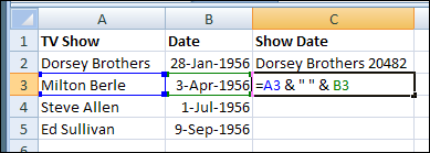
Last Friday, January 8th, would have been Elvis Presley’s 75th birthday. Sadly, he died in 1977, so he never had a chance to work with Microsoft Excel. Otherwise, he might have sung “A Little Less Concatenation”, instead of “A Little Less Conversation.”
Continue reading “Elvis Sings Excel: A Little Less Concatenation”