It’s Price Book publishing week for one of my clients, and we’ve been making lists, and checking them twice. Or 3 or 4 times, or more!
When comparing the new prices to the previous prices, an Excel AutoFilter comes in handy. You can select the same product or model in each workbook, and easily compare item details.
Yes, the widget prices went up a bit this year, so that’s why the assembled parts cost a bit more.
There are written steps and a video below, that show how to use the AutoFilter feature, and workarounds for a problem
Record Count in the Status Bar
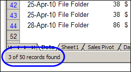
Sometimes when you select records with an AutoFilter, the record count appears in the Status Bar, at the bottom left. In this example, I was working with a small table, with 50 records, and only one column had a formula.
I selected File Folder in the Product column, and the Status Bar showed that 3 of the 50 records contained that product. So far, so good.

Status Bar Shows Filter Mode
Then I added another record to the table, and selected a different product from the AutoFilter drop down list. This time the Status Bar showed the rather unhelpful message, “Filter Mode”, instead of the record count.

Excel 2007 seems to handle this better, but in Excel 2003, and earlier versions, you might see “Filter Mode” if there are more than 50 formulas in the list.
When you apply an AutoFilter, the formula recalculate. If there are lots of formulas to calculate, Excel shows a “Calculating %” message in the Status Bar, so you’ll have something to entertain you while you wait.
Unfortunately, the “Calculating %” message interferes with the record count message in the Status Bar. If the record count message is interrupted, it shows the “Filter Mode” message instead.
You can’t change this behaviour, but there are a couple of workarounds that you can use to find the record count.
Use AutoCalc Instead
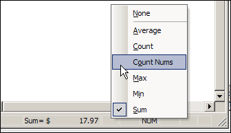
If the Status Bar shows “Filter Mode”, you can get the record count from the AutoCalc feature instead.
- Right-click on the Status Bar
- In the pop-up menu, click Count Nums
- Click on the column heading for a column that contains numbers (and no blank cells within the list)
You’ll see the count of visible numbers in the AutoCalc area of the Status Bar.

Use the SUBTOTAL Function
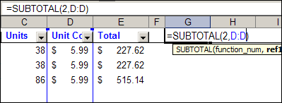
If you’d rather have the record count show up automatically, you can use the SUBTOTAL function. It ignores the filtered rows, and calculates based on the visible rows only.
For example, with numbers in column D, this formula, with 2 as the first argument, will calculate the COUNT of visible numbers:
=SUBTOTAL(2,D:D)

If you want to count items in a column that contains text, use 3 as the first argument, and subtract 1 from the result, to account for the heading cell.
=SUBTOTAL(3,B:B)-1
Watch the Excel AutoFilter Video
In this very short video you can see my Excel AutoFilter experiment, and watch the Filter Mode message appear in the Status Bar.
There are no ruggedly handsome math teachers in this video, but it’s fun-filled and action-packed!
There are more Excel AutoFilter Tips on my Contextures website.
___________

Thanks for that Derbra. It’s been giving me grief for a while now. Using the SUBTOTAL function is perfect. Tony
You’re welcome Tony! Thanks for letting me know that the SUBTOTAL solution works for you.