
There are instructions on my Contextures website for using a combo box with data validation cells. Click on a cell that contains a data validation list, and the combo box appears.
Author: Debra Dalgleish
Allow Only Specific User to Change Excel List
Way back in April, I wrote about the Excel VBA code to automatically add new items to a Data Validation drop down. It’s an easy way to update a list as you work, so the latest items are always available for users.
Last week, someone wrote and asked how to modify that code, so only a specific user could add new items. Everyone else should see a message that says they aren’t permitted to add items.
This technique isn’t foolproof, and anyone who’s determined to circumvent it would be able to. But, it’s a good way to remind people that they can’t update the list without permission.
Identify the User
One way to find out who’s trying to add a new item, is to check the user name that’s entered in the Microsoft Office application.
After you install Office, you can personalize it in Excel Options, in the Popular category, by entering your name in the User Name box.

In Excel VBA, you can create variables to capture that user name, and the name of the authorized user:
    Dim strAuth As String
    Dim strUser As String
    strAuth = "Debra Dalgleish"
    strUser = Application.UserName
Block Non-Authorized Users
After you figure out who the user is, you can block them from doing something. In this workbook, we want to block all but one user from adding new items.
    If strUser <> strAuth Then
        MsgBox "You do not have authority to add Work Order numbers. " _
            & vbCrLf _
            & vbCrLf _
            & "Please check with Administrator before continuing."
        GoTo exitHandler
Remove the Added Item
The above code will block people from adding the new item to the data validation drop down, but doesn’t prevent them from typing the new item in the data validation cell. With another line of code, you can undo the invalid entry that they made.
        Application.Undo
        GoTo exitHandler
Disable Events
Because the code might make a change on the worksheet, you’ll have to turn off the EnableEvents property. That will prevent the Worksheet_Change code from running again, while it’s in the middle of running the first time.
At the top of the procedure, add the line to turn off the EnableEvents property.
Application.EnableEvents = False
In the exitHandler, remember to turn EnableEvents back on.
Application.EnableEvents = True
Full Code and Sample File
If you’re interested in seeing the full code, or downloading the sample file, please visit the Contextures website, and read Excel Data Validation – Add New Items – Specific User.
___________
Remove Pivot Table Calculated Field With Excel VBA
Yesterday, I started out with the best of intentions, planning to get some work done, and find a couple of topics for upcoming blog posts.
Then, while sipping my morning coffee and reading the RSS feeds, I clicked on an article about pivot tables.
Continue reading “Remove Pivot Table Calculated Field With Excel VBA”
PowerPivot from Identical Excel Files
You can use the PowerPivot add-in for Excel 2010 to create a report from multiple Excel workbooks or worksheets, by joining the tables using the Primary and the Foreign key, such as ‘ProductID’ in a Sales table and a Pricing table.
Conditional Formatting From Different Sheet
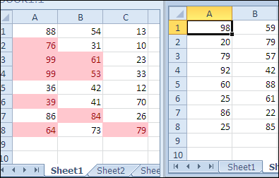
A nice new feature in Excel 2010 is the ability to refer to a different worksheet when creating conditional formatting and data validation. Let’s take a look at how the conditional formatting from different sheet feature works, and create a workaround for older Excel versions.
Continue reading “Conditional Formatting From Different Sheet”
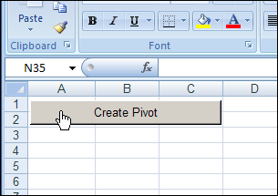
Combine Data From Two Excel Files in Pivot Table
On Monday, Excel MVP Kirill Lapin (aka KL) shared his macro to create a standard pivot table from multiple workbooks (as opposed to worksheets in the same workbook).
I promised you a second pivot table macro, and here it is. In today’s example, Kirill combines data from a sales list and price list, stored in separate workbooks.
The macro combines the data and calculates the selling price for each item, then creates a pivot table from the results.
Continue reading “Combine Data From Two Excel Files in Pivot Table”
Macro Creates Excel Pivot Table From Multiple Files
If you want to create a pivot table from data on different worksheets, you can use a Multiple Consolidation Ranges pivot table. However, that creates a pivot table with limited features and functionality.
Last year, Excel MVP Kirill Lapin (aka KL) shared his brilliant code to create a Union query and build a fully functional pivot table from data on different worksheets.
Continue reading “Macro Creates Excel Pivot Table From Multiple Files”
Print a Customized List of Excel Comments
If you’ve added comments to an Excel worksheet, you have a couple of built-in options for printing the comments.
- Show the comments on the worksheet, and print them as displayed.
- Print the list of comments at the end of the worksheet, on a separate printed page.
Printing Comments Shown on Sheet
Printing the comments on the worksheet is okay if there are only a couple of comments, and you can arrange them so they don’t cover the data.

Print List of Comments
For more than a couple of comments, the list at the end of the worksheet is a better choice.
However, with the built-in list printing option, you just get the cell address and comment, printed in a long, single column.

Create Your Own List of Comments
Instead of using the built-in list of printed comments, you can use a macro to create your own list of comments on a separate worksheet, and print that list.
It’s also a great way to review all the comments on a worksheet, and use sorting or filtering to focus on specific comments.

See the Comment Printing VBA Code
Shown below is the Excel VBA code to create a list of comments from the active sheet, written by Dave Peterson.
For more comment programming examples, including Dave’s code to list all the comments in the entire workbook, see Excel Comments VBA.
The Comment List Code
The ShowComments macro adds a new sheet to the workbook, and lists all the comments, the comment author name, and the comment cell’s value, address and name (if any).
At the end of the macro, the first row is formatted in bold font, and the column widths are autofit.
Sub ShowComments()
'posted by Dave Peterson
    Application.ScreenUpdating = False
Dim commrange As Range
Dim mycell As Range
Dim curwks As Worksheet
Dim newwks As Worksheet
Dim i As Long
Set curwks = ActiveSheet
On Error Resume Next
Set commrange = curwks.Cells _
.SpecialCells(xlCellTypeComments)
On Error GoTo 0
If commrange Is Nothing Then
MsgBox "no comments found"
Exit Sub
End If
Set newwks = Worksheets.Add
newwks.Range("A1:E1").Value = _
Array("Address", "Name", "Value", "Author", "Comment")
i = 1
For Each mycell In commrange
With newwks
i = i + 1
On Error Resume Next
.Cells(i, 1).Value = mycell.Address
.Cells(i, 2).Value = mycell.Name.Name
.Cells(i, 3).Value = mycell.Value
.Cells(i, 4).Value = mycell.Comment.Author
.Cells(i, 5).Value = mycell.Comment.Text
End With
Next mycell
With newwks
.Rows(1).Font.Bold = True
.Cells.EntireColumn.AutoFit
End With
Application.ScreenUpdating = True
End Sub
_____________
Excel VBA: Run Macro on Specific Pivot Tables
 Last week, I posted Bob Ryan’s Excel macro for formatting a pivot table in Classic style. Bob’s macro formats the first pivot table indexed on the active sheet.
    Dim pt As PivotTable
    Set pt = ActiveSheet.PivotTables(1)
Modify the Code
Ideally, you’d only have one pivot table on a worksheet, to prevent problems with overlapping, and Bob’s code would work very well. However, as you know, life in Excel isn’t always ideal!
Let’s look at a few scenarios, and how to modify the macro to deal with them.
Select a Pivot Table
In the blog post comments, Yard suggested a variation on the code, so the macro would run on the selected pivot table, to accommodate worksheets with multiple pivot tables.
If a cell in a pivot table isn’t selected, an “Oops” message would be displayed.
    On Error Resume Next
    Set PT = ActiveCell.PivotCell.PivotTable
    On Error GoTo 0
    If PT Is Nothing Then
        MsgBox "No PivotTable selected", vbInformation, "Oops..."
        Exit Sub
    End If
Thanks, Yard, for your sample code. On a multiple pivot table sheet, the user can control which pivot table is formatted.
Format All Pivot Tables on Active Sheet
Taking that idea a bit further, let’s assume you have a worksheet with several pivot table on it. With Yard’s code, shown above, you could select a cell in one of those pivot tables, and run the macro to format that pivot table only.
But, what if you wanted to format all the pivot tables on that sheet? It would take a while to select each pivot table, and run the macro. Instead, you could modify the code, so it formats all the pivot tables on the active sheet.
    For Each PT in ActiveSheet.PivotTables
        'the formatting code goes here
    Next PT
Format All Pivot Tables on All Worksheets
Finally, what can you do if there’s more than one worksheet with pivot tables? You don’t want to waste time selecting each worksheet, and running the macro to format all the pivot tables on that sheet.
To loop through the worksheet, you could modify the code, so it formats all the pivot tables on each worksheet in the active workbook.
    Dim ws as Worksheet
    For Each ws In ActiveWorkbook.Worksheets
        For Each PT in ws.PivotTables
            'the formatting code goes here
        Next PT
    Next ws
______________
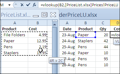
Excel VLOOKUP From Another Workbook
If you’re filling in an order form in Excel, you can use the VLOOKUP function to find the selling price for each item in the sales order. For example, in the screen shot below, the order form is on the Orders worksheet, and a VLOOKUP formula in column D pulls the cost from a pricing table on the Prices worksheet.