
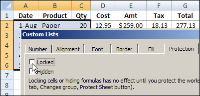
It’s easy to protect a worksheet in Excel, but it’s not so obvious how you leave some of the cells unprotected, to allow changes on a protected worksheet. You can follow this tutorial to learn how to do that, and maybe you’ll even see the weird dialog box heading that I show below.
Author: Debra Dalgleish
Unwanted Files Open Automatically When Excel Starts
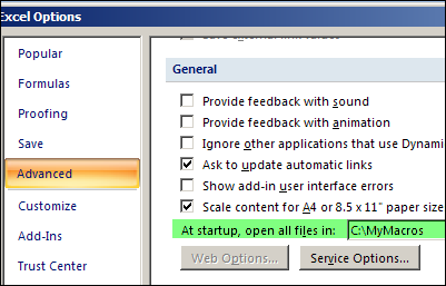
 Do unwanted files open automatically when Excel starts? Perhaps something changed in your computer, and Excel files are opening automatically, and you want to get rid of them. Keep reading, to see where those files might be located, and how to stop them from opening.
Continue reading “Unwanted Files Open Automatically When Excel Starts”
Pivot Table Quick Formatting Macro
My friend and client, Bob Ryan, from Simply Learning Excel, has just published a hands-on, no fluff, Excel book — Simply Learning Excel 2007: Learn the Essentials in 8 Hours or Less.
To celebrate the book launch, I asked Bob to share one of his favourite Excel tips with you, and you can read Bob’s answer below.
Bob’s Pivot Table Macro
Bob Ryan’s top Excel tip:
Some time ago, I was getting ready to train a group of people about PivotTables. As I was documenting the steps, I started feeling more and more annoyed at the number of steps it took to create the kind of PivotTable I typically use.
So, I wrote a macro to automate the steps. (I also submitted a suggestion to Microsoft to allow users to create a customized standard/default PivotTable, but I don’t see it in Excel 2010.)
I wanted to share this macro, but since my website is generally geared to folks who don’t know about or need macros (yet), I asked Debra if I could be a guest writer, and she kindly agreed.
A final note: While I appreciate Debra’s willingness to share this information on her site, the content really belongs to her because most of this information came from her books, website, and/or her personally. I hope you find this useful.
What the Macro Does
Once you insert a PivotTable and enter a field(s) into the Values area, the code does the following to PivotTable(1) on the active sheet:
- Applies the Classic PivotTable display, with gridlines and no colors (I like this so I can Copy the PivotTable and Paste Special Values and Formatting.);
- Ensures that only data that still exists in the data that drives the PivotTable will appear in the PivotTable dropdown lists.
- Sets all fields to ascending order with no subtotals, including fields that are not in the Row Labels or Column Labels areas, and;
- For the data field(s) in the Values area, changes the setting to Sum, changes the number format, and, if the field in the Values area is named “Amount” or “Total Amount” it shortens the label in the PivotTable to “Sum Amt” or “Sum TtlAmt” respectively.
Download the Sample File
You can view the pivot table formatting macro code, and download Bob’s Format Pivot Table Macro sample file.
The file is zipped, and in Excel 2007 format. Because it contains a macro, you’ll have to enable macros when you open the file.
Watch the Video
Thanks, Bob, for sharing your pivot table macro!
To see how much time you can save by using a macro to format a pivot table, watch this video.
It took me a couple of minutes to manually format the Excel pivot table, and change some of the pivot table options, and just a couple of seconds to do all the same steps with Bob’s macro.
Note: If you record your own pivot table formatting macro, follow Bob’s example to add variables, so the macro works on any pivot table, no matter what the field names are, or where it’s located.
About the Author
Robert Ryan, MBA, CPA is a long-time passionate user of Excel, the author of “Simply Learning Excel 2007: Learn the Essentials in 8 Hours or Less,” a unique step-by step book designed for basic to intermediate users, and the host of “Ask the Author… LIVE!™” where Bob answers questions from readers of his book in live WebEx sessions at no extra cost.
_________________
Excel Conditional Formatting Examples
 This week, there were a couple of Excel conditional formatting questions in the blog comments.
- Ron asked about changing the font colour for the highest, second highest and lowest values.
- Guido wants to highlight values that aren’t multiples of another cell’s value.
I’ll answer the questions here, so they’re easier to find. Maybe you’ve encountered similar conditional formatting problems, and this will help.
Change Font Colour for Top 3 Values
The first question is from Ron, who wants to change the font colour, instead of the fill colour:
I am trying conditional format a range of three cells where the FONT of the highest value in the range will be in Red follow by Blue and Green. I know it can be done using cell fill but, with a large spread sheet, it will look like dog’s breakfast. Any help would be appreciated. Also can this be done across worksheets (i.e. three different worksheet in the same file)
Ron didn’t say that the three cells were adjacent, in the same row, but I made that assumption in my example, shown below.

To find the highest, second highest, and lowest values for cells C2:E2 with a worksheet formula, you could do the following:
- To find the highest value, use MAX =MAX($C2:$E2)
- To find the second highest value, use LARGE =LARGE($C2:$E2,2)
- To find the lowest value, use MIN =MIN($C2:$E2)
The column references are absolute, so that all 3 cells in the row will refer to the same range.
You can use the same formulas in conditional formatting, compared to the active cell, and add the font formatting for each formula.
Format the Highest Value
To set up the conditional formatting for the highest value:
- Select cells C2:E6, with C2 as the active cell
- On the Excel Ribbon’s Home tab, click Conditional Formatting, and click New Rule
- In the New Formatting Rule dialog box, under ‘Select a Rule Type’, click ‘Use a formula to determine which cells to format’
- In the formula box, type the MAX formula: =C2 = MAX($C2:$E2) The first reference to C2 is relative, so each cell will check its value compared to the MAX in the $C2:$E2 range.
- Click Format, and on the Font tab, select Red as the font colour, then click OK, twice, to close the dialog boxes.

Now the highest values are highlighted in each row.

Format the Second Highest Value
To set up the conditional formatting for the second highest value:
- Select cells C2:E6, with C2 as the active cell
- On the Excel Ribbon’s Home tab, click Conditional Formatting, and click New Rule
- In the New Formatting Rule dialog box, under ‘Select a Rule Type’, click ‘Use a formula to determine which cells to format’
- In the formula box, type the LARGE formula: =C2 = LARGE($C2:$E2,2)
- Click Format, and on the Font tab, select Blue as the font colour, then click OK, twice, to close the dialog boxes.
Format the Lowest Value
To set up the conditional formatting for the second highest value:
- Select cells C2:E6, with C2 as the active cell
- On the Excel Ribbon’s Home tab, click Conditional Formatting, and click New Rule
- In the New Formatting Rule dialog box, under ‘Select a Rule Type’, click ‘Use a formula to determine which cells to format’
- In the formula box, type the MIN formula: =C2 = MIN($C2:$E2)
- Click Format, and on the Font tab, select Green as the font colour, then click OK, twice, to close the dialog boxes.
Now the highest value in each row is highlighted in red, the second highest is blue, and the lowest is green.

Conditional Formatting From Another Worksheet
To answer the second part of Ron’s question — conditional formatting won’t let you refer to cells on a different worksheet, or in a different workbook.
However, you can refer to a workbook level named range that’s on a different worksheet, but that wouldn’t help in the example shown above.
For example, you could highlight all the cells on Sheet1 that are higher than the maximum allowed, if the maximum is on Sheet2, in a range named MaxAmt.
=C2>MaxAmt
And here’s another example of referring to a named range in conditional formatting.
Highlight Cells That Are Not a Multiple of Another Cell
The next conditional formatting question came from Guido:
need conditional formatting based on the multiple of the number oin another cell. How to do that?
For ex: in the formatted cell can only be the multiple of the number in the other cell, otherwise it colours for ex red
To check this on the worksheet, you could use the MOD function:
=MOD(D2,C2)
The MOD function returns the remainder after a number is divided by divisor. If the result is zero, then D2 is a multiple of C2.
Highlight the Non-Multiples
Shown below is the sample data for this conditional formatting example.

To add the conditional formatting, and highlight the non-multiples in column D:
- Select cells D2:D6, with D2 as the active cell
- On the Excel Ribbon’s Home tab, click Conditional Formatting, and click New Rule
- In the New Formatting Rule dialog box, under ‘Select a Rule Type’, click ‘Use a formula to determine which cells to format’
- In the formula box, type the MOD formula: =MOD(D2,C2) <> 0
- Click Format, and on the Fill tab, select Red, then click OK, twice, to close the dialog boxes.
Now the non-multiples in column D highlighted in red.

More Excel Conditional Formatting Examples
There are more Excel conditional formatting examples on the Contextures website.
______________
Ignore Blank Problems in Excel Data Validation
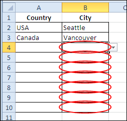
In Monday’s blog, you saw how to make simple dependent data validation drop down lists. After creating the drop downs, you added some flexibility by using the IF function in the data validation formula. See a couple of problems that can occur when you refer to other cells in your data validation, and those cells are blank.
Continue reading “Ignore Blank Problems in Excel Data Validation”
Different Drop Down Lists in Same Excel Cell
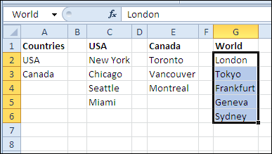
You can use data validation to create drop down lists in Excel. With a bit of Excel magic, you can create dependent drop down lists, so the selection in one drop down controls what appears in the next drop down. You’ll see different drop down lists in the same cell!
Continue reading “Different Drop Down Lists in Same Excel Cell”
Highlight Current Month Birthdays in Excel
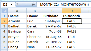
August seems to be a very popular birthday month among my Excel friends. I won’t mention any names here, because most of them are quite elderly, and the shock might upset them. 😉 Anyway, to all of them, and you, if you’re celebrating this month — happy birthday!
Continue reading “Highlight Current Month Birthdays in Excel”
Excel LARGE and FLOOR Functions for Shark Week
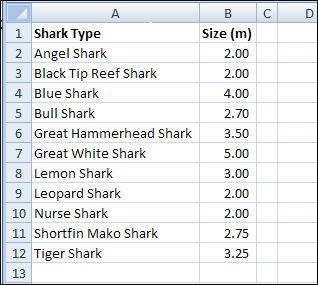
It’s Shark Week on the Discovery Channel, so here are a couple of handy Excel functions you can use in case of a shark attack. Of course, if you stay home and watch television, you should be safe. The infamous land shark rarely attacks.
Continue reading “Excel LARGE and FLOOR Functions for Shark Week”
Built-In Excel Data Form Tips and Quirks
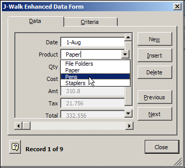
Someone emailed me last week about problems with a range named Database. For reasons known only to the hamsters that operate my brain wheels, that reminded me of Excel’s Data Form.
It’s a built-in data entry tool, that lists all the fields in a table, with entry boxes for some fields, and the formula results showing. You can scroll through the records, or find specific records, based on criteria.
Continue reading “Built-In Excel Data Form Tips and Quirks”
Combine Cells in Excel Without Concatenate
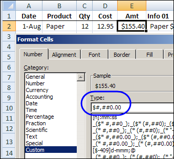
Good news, if you’re spelling challenged — or too lazy to type long words. You can combine cells in Excel, without CONCATENATE function. Keep reading, to learn the easy way to combine cells, and add some fancy formatting to the dates and numbers.
Continue reading “Combine Cells in Excel Without Concatenate”