What’s a quick way to combine the items in two table? For example:
Table A has 3 items – Sugar, Coffee and Milk.
Table B has 2 items – Cans and Sticks.
Combine Table Items
How can you create a third table that has all the Table 1 items combined with each of the Table 2 items?
Sugar – Cans, Sugar – Sticks, etc.
third table has all item combinations
Use MS Query
I’ve done this type of item combining with programming before, but this time I used Microsoft Query, to do the work for me.
Add the two tables to the query, with no join line between them, and the results show each item in table 1 connected to each item in table 2.
two tables in MS Query with no join
Read the Details
To see the details for setting this technique up, and refreshing the results table, please visit the Cartesian Join in Excel Using MS Query page on my Contextures website.
The instructions on that show all the steps for creating the MS query, and then sending the query results to Excel, and finally, refreshing the table if the source data changes.
You can mock me if you want to, but every year I use my Excel Christmas planner to keep track of all the things I want to do, over the holiday season.
Holiday Budget sheet in Excel Holiday Planner Workbook
Where Are the Gifts?
I make a few tweaks to the planner every year, and in this year’s version there is a column to note where you hid a present, after you’ve brought it home.
That should prevent those Christmas Eve panics, while you try to find everything. Not that I’ve ever gone through that – I’m only thinking of you! 😉
Gift Ideas list in Excel Holiday Planner
Black Friday Shopping Plan
This year, the stores are even advertising Black Friday and Cyber Monday sales in Canada, so I’ll be able to use the Black Friday planning sheet, to find a few bargains.
Based on the prices that you enter, the worksheet calculates which store has the best price for each item, and which store has the most deals.
Note: If prices are the same at multiple stores, the first store will be shown in the “Best Price” column.
Price Comparison shopping list in Excel Holiday Planner
Download the Excel Christmas Planner
To download the file, you can visit the Excel Christmas Planner page on my Contextures website.
Happy Thanksgiving, and good luck finding those awesome Black Friday sales tomorrow and in the Cyber Monday sales!
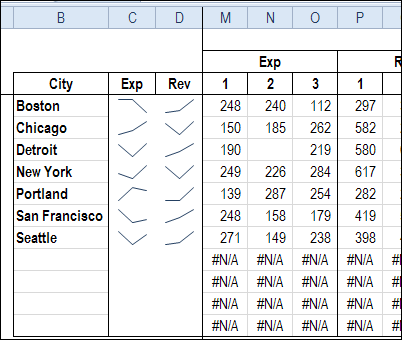
Do you use the sparklines that were introduced in Excel 2010? Last week, I was building a dashboard, and wanted to show sparklines for expenses and revenue.
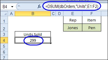
If you need to get a total in Excel, based on criteria, there are a few different ways that you could do it. Today, we’ll take a look at how DSUM and Excel Tables sum with multiple criteria.
Steve emailed me this week, to see if I could help with a lookup problem. He needed to find a discount rate in a lookup table, based on a product code and a date range.
Here is how I solved the problem in Excel 2010 (using fake data), and please let me know if you have a different solution.
Product Pricing Sheet
On a separate sheet, there is a list of products and their prices. This list is formatted as a named Excel table – tblProducts. The two columns in the table are also named – ProdCodeList and ProdPriceList.
Promotions Sheet
On another sheet, there is a list of the promotions that have been offered. This table is named tblPromotions, and each column is also named. We’ll use those names in the formulas.
In this table, I added an ID column at the left, and entered a unique number in each row. The existing Promo Code column has text entries, and for my solution I needed a numeric ID in each row.
Promotions table with ID column at left
Orders Worksheet
On the Orders sheet, a record is created for each new order, with the order date, product code and quantity entered. This table is named tblOrders.
NOTE: Because the formulas are being created in a table, you’ll see column references, like [@Qty], instead of cell references.
You can use an INDEX / MATCH formula to get the product price, based on the product code:
This formula returns a number from the PromoID column, if a promotion is found that matches the criteria:
Promo start date is on or before the order date
Promo end date is on or after the order date
Promo product code matches the order product code
If no matching promotion is found, the sum will be zero. Otherwise, the Promo ID will be the sum.
NOTE: This solution depends on there not being any overlaps in dates for a product promotion. Each promotion ends before another one for the same product begins.
Find the Promo Code
Once the Promo ID has been found, the Promo Code can be looked up, using INDEX and MATCH, based on the Promo ID.
Recently, I enrolled in an online Infographics and data visualization course, and the classes started last week. In one of my homework assignments, I used this trick to link pivot chart title to report filter.
To make data entry easier, add a drop down list on an Excel worksheet. That way, people can choose from the list, instead of typing a product name. If you want to allow other entries with Excel drop down list, follow the steps below, to enable that option.
Recently, my daughter, Sarah, broke her foot, and has had two surgeries, with orthopaedic specialists trying to put all the pieces back together.
I stayed with her for a few days after the latest surgery, to help her out.
One night, just as I was dozing off, I got a message on my iPhone. It was my daughter, texting from the next room.
“Are you still awake?”
“Yes, what do you need?”
“I need help with Excel.”
That made me laugh, and I went in to see what help she needed.
Event Planning with Excel
Sarah is the event planner at Movember Canada, and is organizing launch parties for this year’s Movember events, across Canada.
“During November each year, Movember is responsible for the sprouting of moustaches on thousands of men’s faces, in Canada and around the world. With their “Mo’s”, these men raise vital funds and awareness for men’s health, specifically prostate cancer and male mental health initiatives.”
Of course, event planning is more difficult when you’re confined to your bed, but she’s been going non-stop, despite her injuries.
Apparently the surgical staff had to pry the phone from her hand in the last seconds before she was wheeled into the operating room. Now that’s job dedication!
Excel List of Invitees
Sarah had a list of invitees to the Movember events, and was trying to match email addresses with a short list of people who had not responded to their invitations.
The short list did not include the city name, and she wanted to pull that data from the original list.
Here, using some fake data that I created, is an example of the Excel worksheet, with the long list, and short list.
Solving Problem With Index and Match
Like many other Excel problems, this one can be solved with a combination INDEX/MATCH formula.
The MATCH function finds the email in the original list, based on an exact match
The INDEX function pulls the City from that email address’ row.
INDEX/MATCH Formula
In cell J4, I entered the following formula:
=INDEX($D$4:$D$1000,MATCH(I4,$E$4:$E$1000,0))
The formula looks for the city in column D, in the row where the matching email address was found in column E.
Copy Formula Down
Next, I copied the formula down to the last row in the short list, and all the cities showed up in the short list.
Finally, I copied the City cells in the short list, and pasted them as values, because the formulas weren’t needed any more.
Back to Sleep
It only took a couple of minutes to fix my daughter’s Excel problem, and she thanked me for coming to the rescue.
It warms a mother’s heart to know that her children grew up to be productive adults, who use Excel every day. Sarah might not remember that formula later, but that will give her a reason to call me the next time that she’s stuck in Excel.
After helping out, I headed back to the guest room, and fell asleep. I’m not sure how much longer Sarah kept working, but probably way too long.
And if you’re growing a moustache in support of Movember, please let me know!
When you create a chart in Excel 2010, you can select one of the chart types on the Ribbon’s Insert tab. Microsoft Excel won’t let you select two chart types at the same time though.