Category: Excel VBA

Naming Excel sheets – how hard can it be? Last month, we looked at sheet names, and saw the problems that were caused by using an apostrophe. This week, I found another sheet name problem.

Macro Creates Sales Rep Sheets

Someone, let’s call him Mr. X, contacted me about one of my sample worksheets — Create New Sheets from Filtered List.

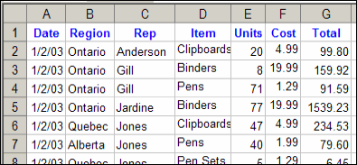
The file has a macro that creates individual sheets for each sales rep, filtering data from a master sheet, like the one shown below.

Second Time Around

Mr. X said he could run the macro once, then got an error the next time he tried to run it. His email also included those dreaded words, “I made some changes.”

Unfortunately, there was no clue as to what those changes were, but at least he attached the problem file.

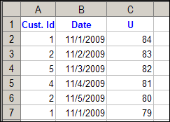
Instead of Rep names, he wanted to created a worksheet for each customer ID.

Sheets with Number Names

Sure enough, the macro created all the sheets, without problems, the first time it ran.

Then, as promised, I got an error the second time that it ran.

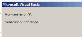
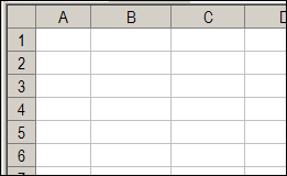
And mysteriously, the Data sheet had been cleared.

The Numbers Game

What happened? Well, the code runs though the list of Customer ID numbers, and if a sheet doesn’t exist for that number, it creates one.

If the sheet does exist, it clears the sheet, then adds the new data.

When the code got to customer ID 1, instead of clearing the “1” sheet, it cleared the first sheet, Data, which has an index number of 1.

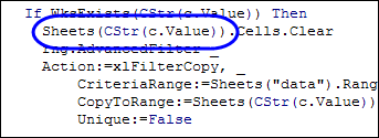
To fix the problem, I changed the c.Value reference in the code to CStr(c.Value)).

Now, instead of looking for the sheet with an index number of 1, it looked for a sheet with a name of “1”.

Watch the Numbers

If you use numbers as sheet names, such as a sheet for each day of the month, be careful how you refer to those sheets in your code.

You don’t want to end up like Mr. X, with blank sheets, and error messages!
______________

If you create an Excel add-in, and offer it for sale, how do you decide what to charge for that utility?

How Do You Price Software?

What is your pricing strategy?

• Do you check out the competition and price your utility in the same range?
• Do you crunch a pile of numbers in Excel, and base your price on the results?
• Do you just make a wild guess, and put that price on the sticker?
• Or something else?

Product Pricing Guide

To help you with pricing, you can get a copy of the book:

• Don’t Just Roll the Dice: Usefully Short Guide to Software Pricing

It’s written by software developer, Neil Davidson, of Red Gate Software.

Your local library might have a copy of the book, that you could borrow. Or, check your local bookstore, to see if they have it in stock.

Or, if you’d like your own paperback copy of the book, or a digital copy for your Kindle reader, you can buy the book on Amazon.

Author’s Experiences

The book explores the economics and psychology of pricing, and the author cites his own experiences (good and bad) with software pricing.

It’s easy to read, with clear explanations and examples, and ends with a product pricing checklist.

It also has this sensible advice: “Try out your pricing and see what happens.”

Excel Add-Ins

If you buy someone else’s Excel utilities, there are steps on my Contextures site, for how to Install and Use Excel add-ins.

Usually, Excel add-ins are installed in Excel’s default folder for Add-ins. My instructions show you how to find that folder, or choose a different folder, if you prefer.

Free Excel Add-ins

I use a few free add-ins that make Excel even better, and asked other people what free add-ins they use, and would recommend.

I compiled a list, starting with my favourites. Maybe you’ll see a few that you can download and install, and make working in Excel a bit easier.

Click here to see my list of recommended free Excel add-ins.

More Excel Resources

For the latest Excel courses, Excel books and Excel add-ins and tools, go to the Debra’s Excel Picks page, on my Contextures website

I’ve listed my top picks for Excel courses, add-ins, books, and Excel tools. See how to raise your skills to expert level, and get tools that will save you time

______________

Even though an Excel workbook doesn’t contain any macros, sometimes when you open a file, a security warning appears.

Macros Disabled

For example, in the screen shot below, there is a warning above the Excel formula bar:

• Excel Security Warning – Macros have been disabled

Why Security Warnings Appear

These security warnings can show up if:

• you recorded a macro in the Excel workbook
• later, you deleted the Excel macro

A module is automatically created to store a recorded macro, but that module is not automatically deleted, when you delete the recorded macro.

Delete the Empty Module

Follow the steps in the video below, to delete the empty modules in the workbook.

• Warning: As a precaution, you should make a backup copy of the file, before you remove any code.

Doing that should prevent the security warning from appearing again, the next time you open the workbook.

Note: To see the written steps, go to the Excel Macros – Frequently Asked Questions page on my Contextures site.

______________

Some people like an Excel workbook that’s locked down, so they can’t accidentally mess anything up. They just want to go to the data entry section, put in their data, and get out alive.

Protect or Unlock?

Other people hate Excel workbooks that are protected. Maybe they know a bit more about Excel, and are comfortable making changes.

Or, they’ve been assigned to manage a workbook, and don’t want to bother with worksheet protection, because it slows them down.

Give the Users Control

One of my clients has plants all over the world, and we’ve made a similar data collection workbook for each plant.

On the last sheet of the workbook, I’ve added a drop down list, where the user can select TRUE or FALSE, to lock the worksheets.

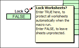
• If the setting changed to FALSE, a macro runs, to unprotect all the worksheets.
• If the setting is changed to TRUE, all the sheets are protected.

The TRUE/FALSE option is a quick and easy way for users to control the workbook settings, and seems to be working well.

The Code

There’s code on the worksheet module that runs when the Lock cell’s value is changed. To see the code, right-click on the sheet tab where the drop down list is located, and click View Code.

Here’s the bit of code that checks the Lock cell, and protects or unprotects the sheets. In the sample file, there is the full code, and another example that protects or unprotects with a password.

If Target.Address = wsListsAll.Range(“Lock”).Address Then
For Each ws In ThisWorkbook.Worksheets
If bLock = True Then
ws.Protect
Else
ws.Unprotect
End If
Next ws
End If

Download the Sample File

If you’d like to see all the code, you can download the sample file from the Worksheet Protection Selector page on my Contextures website.

On that page, scroll down to the Download section, and you’ll see a link to the file.

The file contains macros, so you’ll have to enable them to test the code.
_______________________

If you add comments to an Excel worksheet, you might want to include those comments when printing. There are a couple of built in options for printing comments, but neither is ideal.

We’ll look at those options first, then a numbering system, that’s similar to numbered footnotes.

The Built In Options

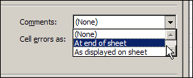
In the Page Setup dialog box, on the Sheet tab, there are 3 options for printing the comments:

• (None)
• At end of sheet
• As displayed on sheet

Print At End of Sheet

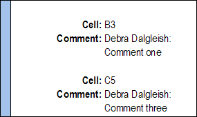
If you select At end of sheet, a separate page of comments prints, listing the cell address, commenter name and comment text.

As Displayed on Sheet

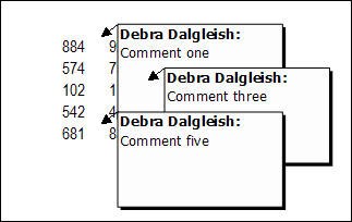
If you select As displayed on sheet, the comment that are currently visible on the worksheet will print, exactly as they appear on screen.

That might work if there are a couple of comments that you want to show, and can arrange them over an empty space. Otherwise, you’ll end up with a jumbled mess of comments, covering your data.

Add Numbers to Cells With Comments

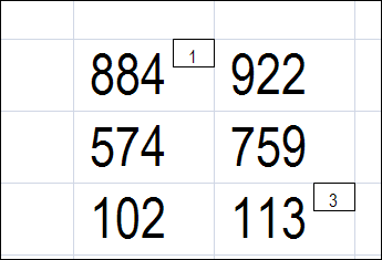
Instead of using either of the built in options to print comments, you could use a bit of programming to add a tiny number at the top right of each cell that has a comment. Here’s a close up view of the numbered cells.

List the Numbered Comments

With another bit of programming, you can create a numbered list of the comments, with other details, such as range name, cell value, cell address and comment text.

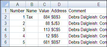
This list is on a separate worksheet, that you can print when you print the sheet with comments.

Download the Sample File

To download the sample file for Excel 2003 or Excel 2007/2010, go to the Number and List Comments section on the Comments programming page. There’s sample code to add numbers, remove numbers and list the comments, and a zipped sample file that you can download.

The Excel 2003 numbering code didn’t work well in Excel 2007. The numbers didn’t appear in some boxes, and the boxes didn’t line up correctly in the cells. So if you’re using Excel 2007, be sure to download that version’s sample file

Both files contain macros, so you may get a warning when you open them. Enable the macros if you want to run the code.
__________

Last week one of my clients asked for a bit of help, so I sent a workbook with some sample code to tackle the problem. It was just what he needed, so my client wanted to copy the code from the sample file, into his own workbook.

Unfortunately, he wasn’t sure how to do that, and asked for a bit more help.
A quick way to copy code is to drag a module from one workbook to another, in the Visual Basic Editor. In this example, the code is in VBACodeCopy.xls and will be copied to MyForm.xlsm.

1. Open both workbooks
2. On your keyboard, hold the Alt key, and press the F11 key, to open the Visual Basic Editor
3. In the Project Explorer window, find both workbooks.
4. In the workbook with the code, click the + sign to view the list of Modules
5. Click on the module that you want to copy, and drag it over the project where you’d like the copy placed.
6. Release the mouse button, and a copy of the module will appear in the workbook. It will automatically create a Modules folder, if necessary.

Copy and Paste Excel Code

If you only want some of the code on a module sheet, or to copy code from a worksheet or workbook module, you can copy and paste the Excel code.

Watch the Video

To see the steps for copying an entire module, you can watch this short video.

________________

In my workbooks, I sometimes add buttons to run macros. Usually, they’re for navigation to the next or previous sheet, or to run a macro that’s specific to the contents of the worksheet.

In this example, I’ve got two macros in the workbook – one that takes you to the next sheet in the workbook, and one that takes you to the previous sheet.

So, if you’re on the second sheet, you can click the Next button to go to the third sheet. Or, click the Back button to go to the first sheet.

Update: I’ve added a video, about halfway down the page, to show the steps.

Add a Button

• On the Ribbon, click the Developer tab
  • Note: If the Developer tab isn’t visible, click the Office Button, then click Excel Options. Click the Popular category, then add a check mark to Show Developer tab in the Ribbon.
• In the Controls group, click Insert, to see the controls from the Form toolbar and the Control Toolbox.
• In the Form Controls section, click Button.

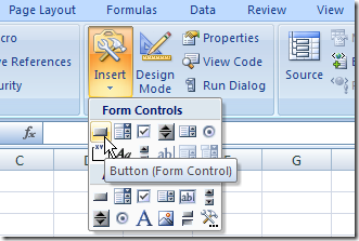
• Click on the worksheet to add a button, or drag on the worksheet to add a button of a specific size.
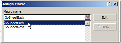
• In the Assign Macro dialog box that opens automatically, click on the name of a macro to select it, then click OK

Format the Button

While the button is still selected, you can change its caption and add some formatting.

• To change the button’s caption, select the existing text, and type a caption to replace it. The border around the button will have diagonal lines when you’re editing the text

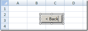
• Click on the border of the button, to select it. The outline should change to a dotted pattern, as you can see in the next screenshot.

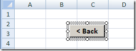
• On the Ribbon’s Home tab, use the font formatting buttons, such as Bold and Font Size, to change the appearance of the button.

Use the Buttons

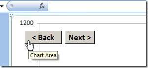
After you’ve added the Back button, repeat the steps to create a Next button. Then, copy the two buttons to any worksheets or chart sheets in the workbook.

To move through the sheets, click either the Back or Next button on any sheet.

Video: Add Worksheet Navigation Buttons

This video shows how to add the buttons, and align them. Then it shows how to copy the buttons to other worksheets.

NOTE: This video does NOT show the steps for writing the Excel macros. Those are in the sample file that you can download.

The Navigation Code

Here’s the code that I used to make the buttons select the next or previous sheet.

Sub GoSheetNext()
Dim wb As Workbook
Dim lSheet As Long
Set wb = ActiveWorkbook
lSheet = ActiveSheet.Index
With wb
  If lSheet = .Sheets.Count Then
    .Sheets(1).Select
  Else
    .Sheets(lSheet + 1).Select
  End If
End With
End Sub
'=================================
Sub GoSheetBack()
Dim wb As Workbook
Dim lSheet As Long
Set wb = ActiveWorkbook
lSheet = ActiveSheet.Index
With wb
  If lSheet = 1 Then
    .Sheets(.Sheets.Count).Select
  Else
    .Sheets(lSheet - 1).Select
  End If
End With
End Sub

Get the Sample File

To get an Excel sample file with buttons to navigate to the previous or next worksheet, go to the Worksheet Macro Buttons page on my Contextures site. The zipped Excel file is in xlsm format, and contains macros.

Update: There is a newer version of the code on this Add Navigation Buttons blog post.

________________

Today’s challenge was to create a table of contents in Excel, for a downloaded price list.

Section Headings

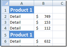
The data came from Crystal Reports and had formatting on the section headings.

Some of the headings were repeated, but we didn’t want the TOC to include the duplicates.

Heading Cell Format

I’ve created a table of contents based on sheet names, in other workbooks, but hadn’t tried to index a sheet’s contents.

In this case, all the heading cells were blue, so I decided to write a macro that would create a TOC entry for any blue cell.

A quick test in the Immediate window showed me the colour index — 42.

What Excel VBA Macro Code Does

The macro that I wrote does the following steps:

• checks for a TOC sheet
• deletes the old one, if it exists
• then creates a new TOC sheet
• first instance of each heading is added to the TOC sheet
• adds a hyperlink to the cell where that heading is located.
• creates an AutoFilter for the list

The price list has a few hundred product categories, so that Autofilter makes it easier to find the product that you want.

The CreateHyperlinks Code

Here’s the Excel VBA code that I wrote, and you can add your own error handling.

You can also download the sample Hyperlink TOC file (Excel 2007 format).

Sub CreateHyperlinks()
Dim c As Range
Dim ws As Worksheet
Dim wsTOC As Worksheet
Dim lRowTOC As Long
Dim lColor As Long
Dim strTOC As String
Dim strHead As String
lRowTOC = 2
lColor = 42
strTOC = "TOC"
strHead = ""
On Error Resume Next
Application.DisplayAlerts = False
Worksheets(strTOC).Delete
Application.DisplayAlerts = True
On Error GoTo 0
Set wsTOC = Worksheets.Add
With wsTOC
  .Name = strTOC
  .Cells(1, 1).Value = "Product"
  .Cells(1, 1).Font.Bold = True
End With
For Each ws In ThisWorkbook.Worksheets
  If ws.Name <> strTOC Then
    For Each c In ws.UsedRange.Columns(1).Cells
      If c.Interior.ColorIndex = lColor Then
        'don't index duplicate headings
        If strHead <> c.Value Then
          wsTOC.Cells(lRowTOC, 1).Value = c.Value
          wsTOC.Hyperlinks.Add _
          Anchor:=wsTOC.Cells(lRowTOC, 1), _
          Address:="", _
          SubAddress:=c.Parent.Name _
          & "!" & c.Address, _
          TextToDisplay:=c.Value
          lRowTOC = lRowTOC + 1
          strHead = c.Value
        End If
      End If
    Next c
  End If
Next ws
wsTOC.Columns(1).AutoFilter
wsTOC.Columns(1).AutoFit
End Sub

___________________

With a bit of programming, you can make it easy for users to enter data in an Excel workbook, and keep them away from the stored data.

Sample Data Entry Form

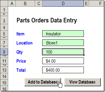
Dave Peterson created a sample workbook with a worksheet data entry form.

Data Entry Features

In the worksheet Data Entry form, there are data validation drop down lists in cells D5 and D7.

The quantity number is typed in cell D9.

After you fill those 3 cells, click the Add to Database button.

A macro runs, and your new record is added at the end of the database, which is a list stored on a different sheet.

View the Stored Records

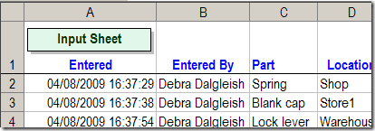
In Dave’s workbook, you could click the View Database button to go to the database sheet, and review or edit the existing order records.

Worksheet Scroll Buttons

In some cases you might prefer to hide the database sheet, to protect the records, but still allow users to view the existing data.

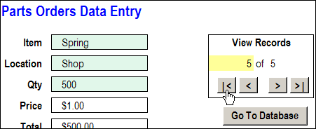
I’ve added a few buttons to Dave’s workbook, to allow users to scroll through the existing records.

Navigation Buttons

The navigation buttons take you to the first, previous, next or last record.

Or, you can type a record number in the yellow cell, to go to a specific record.

Go To Database Button

In the updated workbook, I left the “Go To Database” button on the data entry worksheet.

You could remove that button, and hide the PartsData sheet, if you prefer, so users are less likely to change the data.

Download the Sample File

The zipped sample workbook can be downloaded from the Data Entry Worksheet Form page on my website.

In the Download section, look for Version 2 – Navigation Arrows.

More Articles on the Worksheet Data Entry Forms

New Improved Excel Data Entry Form

How to Customize the Excel Data Entry Form

Delete Orders with Excel Data Entry Form

Check Excel Database Before Adding New Item
___________________________