Last December, Priacta offered free enrollment in Total Relaxed Organization, their online time management course, so I signed up, and worked on the lessons over the Christmas holidays.
It changed the way I work, and almost three months later, I’m still using the techniques that I learned.
The course is based on Getting Things Done, and helps you clear up your workspace and organize your tasks. You can customize the course for the PDA or smart phone that you use, and your preferred task list. I chose Outlook (Excel wasn’t an option) and Blackberry.
The course is in three parts:
- Principles and Preparation
- Collecting and Organizing
- Processing, Reviewing, Doing
The lessons were well organized, and clearly written, with a navigation pane at the left, and lesson content on the right.

The site records the time you spend on the online course, and it took me about 10 hours complete the lessons.
I spent a few more hours offline, cleaning up my office. Telephone coaching was offered at several points during the course, to speed up the process, but I didn’t opt for that.
I’m sure the coaches are fine people, but I didn’t hit any snags where I felt a personal coach would help.
What I Learned
The object is to collect your tasks in a few specific places, such as email, voice mail and inbox, instead of many scattered places, including your memory.
Then, you process what you’ve collected, and work from a prioritized task list, with supporting documents filed away until you’re ready to use them.
For me, this was the most useful lesson, because I used to keep stacks of folders near my desk, for projects I was working on. Now the papers are filed by client name, and I can’t feel their beady eyes burning into me as I work.
That reduces my stress level, because I’m dealing with one task at a time, not trying to juggle several things.
I didn’t like all of the suggestions for changes to Outlook, so ignored much of that. Also, although I chose Outlook during the setup, I substituted my Excel task list, so didn’t follow all the steps exactly.
I was able to categorize, sort and filter things in Excel, but in a slightly different way than you would in Outlook.
Have You Tried It?
I think the first 8 or 9 lessons are always free, and the complete course (23 lessons) is $99 (the site says it’s currently $69). The course might not suit your work style, but if you want to get organized, look at the free lessons and see if you like it.
Have you already tried the course, or something similar? Did you find it helpful, and stick with it?
_________________