
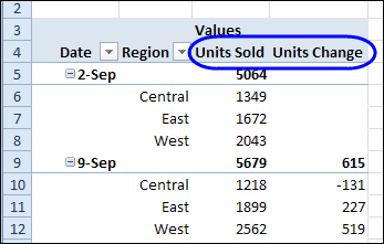
A pivot table is a great way to summarize data, and most of the time you probably use a Sum or Count function for the values. For example, in the pivot table shown below, the regional sales are totaled for each week. We can also use a built-in feature to calculate differences in a pivot table.
Author: Debra Dalgleish
Excel Dot Plot Chart for Stock Prices
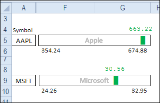
Today we’ll create an in-cell chart that shows the latest price for a stock, compared to its low and high prices. There is a sample file available for download, and a video that shows the steps.
Create Alternating Shaded Rows on Excel Sheet
If you’re using a named Excel table, you can apply a style that shades alternate rows with colour. In the table shown below, the row shading has two rows of grey followed by one row of white.
To create this table style, I duplicated one of the existing styles, and modified the row shading.

If you don’t want to use a table, or table styles aren’t available in your version of Excel, you can still have shaded rows, by using conditional formatting.
Shade Rows With Conditional Formatting
To shade the rows, we’ll use the MOD function in a conditional formatting formula. To see how it works, we can test the MOD function on the worksheet, in column G.
We want a set of 3 rows – two with shading, and then a row with no colour. With the MOD function, we’ll get the remainder, if the row number is divided by 3.
=MOD(ROW(),3)
The result for each row is shown in column G, and is either 0, 1 or 2.

We can shade rows where the result is 0 or 1, and leave the rows with 2 as no fill colour. To check the result of the MOD function, we can add a formula in column H, to see if it’s less than 2.
=G2<2

If the result is TRUE, we can shade the row. I’ve highlighted the TRUE cells in the screen shot above, to show which rows will be shaded.
Columns G and H were just used to test the formula, so I’ll clear those out, before formatting the cells.
Create a Conditional Formatting Formula
To shade the rows, we’ll combine the MOD function and the test of the results, in a conditional formatting formula.
- Select the cells where you want the banded rows to appear. In this example, cells A2:F9 are selected.
- On the Ribbon’s Home tab, click Conditional Formatting, then click New Rule
- For Rule Type, click on Use a Formula to Determine Which Cells to Format
- For the formula, enter =MOD(ROW(),3)<2
- Click the Format button.
- On the Patterns tab, select a colour for shading – light grey was used in this example
- Click OK, click OK

The selected range has two rows of grey shading, followed by a row with no fill colour.

Make the Shaded Rows Adjustable
In the previous example, the numbers 3 and 2 were typed into the conditional formatting formula. To make the shading adjustable, you could enter the numbers on the worksheet, and then refer to those cells in the formula.
On the worksheet, create an input range for the numbers. In this example, the numbers are entered in J1 and J2, and the sum of those numbers is in J3.

Modify the Formula
To change the conditional formatting formula:
- Select a cell in the range where the conditional formatting rule was applied. In this example, cells A2:F9 are selected.
- On the Ribbon’s Home tab, click Conditional Formatting, then click Manage Rules
- Click on the MOD rule in the list of rules, and click Edit Rule
- Change the formula, so it refers to the grey shading number — $J$1, and the total number — $J$3:
- =MOD(ROW(),$J$3)<$J$1
- Click OK, click OK

Test the Shading
To test the interactive shading formula, change one or both of the numbers in J1:J2. The shading on the worksheet should automatically adjust.
In the screen shot below, the numbers were changed so there is one grey row, followed by 2 rows with no fill.

Watch the Video
To see the steps for creating shaded rows on the worksheet, please watch this short video tutorial.
Download the Sample File
To download the sample file, please visit the Conditional Formatting Examples page on my Contextures website. The Excel 2010 / 2007 sample file contains the interactive example.
______________________________
Lock Excel Heading Rows in Place
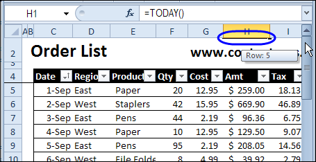
If you want to scroll down the worksheet, and lock the heading rows in place, so they’re always visible, you can use the Freeze Panes command. Be careful though, or you might end up with hidden rows that you can’t get to.
Change Functions With Excel Drop Down List
Last year, I shared a technique for selecting a function name from a drop down list, and that changed the formulas in a summary row on the worksheet.
Select Function Name
For example, from the drop down list in cell C2:
- Choose the MAX function, to see the highest amounts in a lists of sales orders.
- Next, choose the SUM function, to see the total amount in the lists of orders
- Or, choose the COUNT function, to get the total count

This technique runs on formulas, not macros, and is a great way to show different information in a small amount of worksheet space.
It could be perfect for an interactive Excel dashboard, where people can choose the information they want to see.
Watch the Video
I’ve finally made a video that shows how to create this changeable summary, and create a drop down list of functions.
You can watch the video here, and for written instructions, and the sample file download, visit this page: Change Excel Function With Subtotals
As I show in the video, to alternate between functions, such as SUM, AVERAGE or MAX in a summary row, use the Subtotal function in your formulas.
Then, add a drop down list of functions on the worksheet, using the Excel data validation feature. Next, select the function you want, to see those results in the summary.
This technique does not require macros — the formulas create the changing summaries.
________________
Format Excel Worksheet for Troubleshooting
Do you ever get sent an Excel file, and asked to figure out why it’s not working correctly? The odds are that it was created several years ago, by someone who has left the company, and a few other people have “improved” it over the years.
Now it’s a mess, and nobody is sure exactly how it works. It’s up to you to sort it out. Lucky you!
Here’s how I start the troubleshooting process, and you can see the steps in the video below. There are detailed instructions on my Contextures site.
Make a Copy of the Original File
In the screen shot below, you can see a worksheet that is similar to the ones that I troubleshoot. There is a rainbow of colours on the sheet, but they don’t seem to have any significance – they’re just someone’s favourite colours.
I’ll get rid of that rainbow, and colour the cells that contain:
- formulas
- text
- numbers
- data validation
But the first step is to make a copy (or two) of the original file, and store it in a safe place. Don’t make any changes to the file, until you have that backup file safely stored away – you might want to refer to it later, as you dig deeper into the troubleshooting.

Clear All Colour
The next step is to remove all the colour fill from the worksheet, so you can add your own colour scheme.
- Select all the cells on the worksheet
- Choose No Fill as the cell fill colour
When you’re finished troubleshooting, and the worksheet is functioning correctly, you can clear the troubleshooting formats.
Then, add colour to the data entry cells, or other key cells, to help people understand how the workbook should be used.
Colour the Formula Cells
The next step is to find and format the cells that contain formulas.
- On the Ribbon’s Home tab, click the Find & Select command
- Click on Formulas, to select all the formula cells

- Then, use the Fill command on the Ribbon to format the Formula cells. I usually use grey for the formula cells, which indicates that they shouldn’t be changed.
Colour Remaining Cells
Next, you can find and format the cells that contain constants, and data validation, by using the other options in the Find & Select drop down.
- On the Ribbon’s Home tab, click the Find & Select command
- Click on Constants, then format the Constant cells.
- Repeat the steps to format the Data Validation cells, where drop down lists or special rules apply
Colour Constant Numbers
Finally, find and format the cells that contain constant numbers. These might be data entry cells, that you can use in testing the worksheet.
- On the Ribbon’s Home tab, click the Find & Select command
- Click the Go To Special command.
- Select Constants, and check the box for Numbers. Remove the check mark in the Text, Logicals and Errors boxes, then click OK.

- Then, format the constant number cells
Finish Worksheet Formatting
After all the key cells are colour coded, you can add a legend on the worksheet, to show what the colours mean.
Then, get started with the troubleshooting. For example, in the screen shot below, the circled cells contain constants, but they should contain formulas.

Watch the Formatting Video
To see the steps for formatting the different types of cells, you can watch this short video.
___________________
Excel Drop Down Opens At End
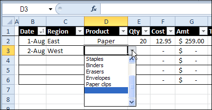
To make data entry easier, you can create a drop down list of items in a worksheet cell. Then, instead of typing a product name in an order list, you can select a valid product name from the list. Sometimes the Excel drop down opens at end of the list, instead of the top. Here’s how to fix that problem.
Update Specific Pivot Tables Automatically
In Excel 2010, you can use Slicers to change multiple pivot tables. However, you might be working in an earlier version of Excel, or you don’t have room for Slicers on your worksheets.
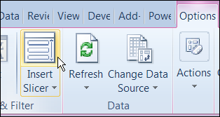
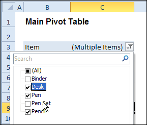
Instead of Slicers, you can use programming to update multiple pivot tables automatically. In previous posts, I’ve shown how you can select items in one pivot table’s Report Filter fields, and the Report Filter fields for pivot tables on the other worksheets will change to the same selections.
Specific Sheet and Pivot Tables
Jeff Weir has written an updated version of the code, which runs much faster than the previous version. You’ll notice the speed difference especially if you’re working with larger pivot tables.
Also, in this version of the code, you can specify:
- any sheets you DON’T want the macro to check
- any specific pivot tables that you DON’T want the macro to synchronize.
For example, only update the pivot tables on Sheet1 and Sheet2, and ignore PivotTable2 on Sheet1.
[Update: Sept 20, 2012] Jeff has made the following changes to the code:
- you can now exclude particular PivotFields, plus if you change a pagefield in any pivot, the code will not only update pagefields to the same settings in other pivots but also change rowfields too.
- added basic error handling so that ScreenUpdating and EnableEvents are restored to TRUE if anything goes wrong.
Jeff is also working on a version of the code for Excel 2010, that promises to be even faster — so stay tuned for that!
[Update: June 16, 2013] Jeff has revised the code, so it uses Slicers if the version is Excel 2010 or later.
Making Code Run Faster
In the previous version of the code, it looped through each master pivot field multiple times, to determine if each pivot item is visible or hidden. The corresponding pivot item in each secondary pivot table was then set to the same setting. The code worked, but it was very slow in larger pivot tables.
The main reason that Jeff’s code is faster is that it iterates through each master pivot field just once, so it can record only the visible items into a dictionary.
Then, for each pivot field in each secondary pivot table:
- All the pivot items are made visible
- Items that are not in the dictionary’s list are hidden.
Also, speed in Jeff’s code is increased because it:
- checks to see if.AllItemsVisible = true. If it is, no need to iterate through either the master or the secondary pivot…it just makes all pivot items in the corresponding secondary pivot fields visible. The old code looped through each pivot item
- doesn’t add items to the dictionary for checking if it has already found all the visible pivot items in the master list.
Modify the Code
If you download the sample file (see instructions below), you can copy the code to your own workbooks.
- To see the code in the sample file, go to the Sales Pivot worksheet, right-click the sheet tab, and click View Code.
- Then, to see the full code, right-click on the procedure name – SyncPivotFields – and click Definition
Here is where you’ll change the sheet names in the SyncPivotFields code:

Here is the section where you’ll change the pivot table names:

Download the Sample File
To download this version of the sample file, with Jeff’s code, please visit the Sample Files page on the Contextures website.
Note: Jeff’s sample file was updated on Sept. 20, 2012, so please download the new version if you have an older copy of the file.
In the Pivot Tables section, look for: PT0029 – Change Pivot Table Fields on Specific Sheets
The file is in Excel xlsm format, zipped, and contains macros. Enable the macros when opening the file, if you want to test the code.
__________________
How to Create a Panel Chart in Excel
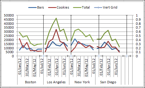
To show a concise, clear summary of data for several departments or cities, you can create a panel chart in Excel. It shows all the data in a single chart, with vertical lines separating the groups.
Edit Excel List Data in Popup Form
If you’re working with a list of data in Excel, you can use Excel’s built-in Data Form to view and edit the data.
Displaying up to 32 fields, it lets you view and edit one record at a time. You can also find and edit records, or add and delete them.
Continue reading “Edit Excel List Data in Popup Form”