Yesterday, in the 30XL30D challenge, we found character code numbers with the CODE function, and used it to reveal hidden characters.
CHAR Function
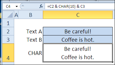
For day 8 in the challenge, we’ll examine the CODE function’s evil twin — the CHAR function.
Excel tips and tutorials

Yesterday, in the 30XL30D challenge, we found character code numbers with the CODE function, and used it to reveal hidden characters.
For day 8 in the challenge, we’ll examine the CODE function’s evil twin — the CHAR function.
 Congratulations! You’ve made it to the first weekend in the 30XL30D challenge, including yesterday’s investigation of the FIXED function.
We’ll take it easy today, and look at a function that doesn’t have too many examples — the CODE function. It can work with other functions, in long, complicated formulas, but today we’ll focus on what it can do on its own, and in simple formulas.
So, let’s take a look at the CODE information and examples, and if you have other tips or examples, please share them in the comments. Wear your secret deCODEr ring, if you have one.
The CODE function returns a numeric code for the first character in a text string. For Windows, the returned code is from the ANSI character set, and for Macintosh, the code is from the Macintosh character set.

The CODE function can help unravel mysteries in your data, such as:
The CODE function has the following syntax:
Results could be different if you switch to a different operating system. The codes for the ASCII character set (codes 32 to 126) are consistent, and most can be found on your keyboard.
However, the characters for the higher numbers (129 to 254) may vary, as you can see in the comparison charts shown here:
Differences between ANSI, ISO-8859-1 and MacRoman character sets
For example, the ANSI code 189 is ½ and for the Macintosh it is O
When you copy text from a website, it might include hidden characters. The CODE function can be used to identify what those hidden characters are.
For example, there is a text string in cell B3, and only “test” is visible — 4 characters. In cell C3, the LEN function shows that there are 5 characters in cell B3.
To identify the last character’s code, you can use the RIGHT function, to return the last character. Then, use the CODE function to return the code for that character.
=CODE(RIGHT(B3,1))

In cell D3, the RIGHT/CODE formula shows that the last character has the code 160, which is a non-breaking space used on websites.
To insert special characters in an Excel worksheet, you can use the Symbol command on the Ribbon’s Insert tab. For example, you can insert a degree symbol ° or a copyright symbol ©.
After you insert a symbol, you can determine its code, by using the CODE function
=IF(C3=””,””,CODE(RIGHT(C3,1)))

Once you know the code, you can use the numeric keypad (not the regular numbers) to insert the symbol. The code for the copyright symbol is 169. Follow these steps to enter that symbol in a cell.
On your laptop, you might need to press special keys to use the numeric keypad function. Check the owner’s manual, for directions. Here’s what works on my Dell laptop.
To see the formulas used in today’s examples, you can download the CODE function sample workbook. The file is zipped, and is in Excel 2007 file format.
To see a demonstration of the examples in the CODE function sample workbook, you can watch this short Excel video tutorial.
_____________
Yesterday, in the 30XL30D challenge, we picked an item from a list with the CHOOSE function, and learned that other functions might be a better MATCH when doing a LOOKUP.
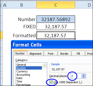
For day 6 in the challenge, we’ll examine the FIXED function, which formats a number with decimals and commas, and returns the result as text.
Continue reading “30 Excel Functions in 30 Days: 06 – FIXED”
Yesterday, in the 30XL30D challenge, we got details on our operating environment, with the INFO function, and learned that it can no longer help with our memory issues. (Neither ours, nor Excel’s!)
For day 5 in the challenge, we’ll examine the CHOOSE function.
Continue reading “30 Excel Functions in 30 Days: 05 – CHOOSE”
Yesterday, in the 30XL30D challenge, we cleaned things up with the TRIM function, and learned that it’s no SUBSTITUTE for calorie counting.
For day 4 in the challenge, we’ll examine the INFO function. Excel Help warns us to be careful with this function, or we could reveal private information to other users.
So, let’s take a look at the INFO information and examples, and if you have other tips or examples, please share them in the comments. And remember to guard your secrets!
The INFO function shows information about the current operating environment.

The INFO function can show information about the Excel application, such as:
In previous versions of Excel you could also get memory information (“memavail”, “memused”, and “totmem”), but those type_text items are no longer supported.
The INFO function has the following syntax:
In Excel’s Help file, there is a warning that you should use the INFO function with caution, because it could reveal confidential information to other users.
For example, you might not want other people to see the file path that your Excel workbook is in. If you’re sending an Excel file to someone else, be sure to remove any data that you don’t want to share!
With the “release” value, you can use the INFO function to show what version of Excel is being used. The result is text, not a number.
In the screenshot below, Excel 2010 is being used, so the version number is 14.0.
=INFO(“release”)

You could use the result to display a message, based on version number.
=IF(C2+0<14,”Time to upgrade”,”Latest version”)

With the “numfile” type_text value, the INFO function can show the number of active worksheets in all open workbooks. This number includes hidden sheets, sheets in hidden workbooks, and sheets in add-ins.
In this example, an add-in is running, and it has two worksheets, and the visible workbook has five worksheets. The total sheets returned by the INFO function is seven.
=INFO(“numfile”)

Instead of typing the type_text value as a string in the INFO function, you can refer to a cell that contains one of the valid values.
In this example, there is a data validation drop down list in cell B3, and the INFO function refers to it.
=INFO(B3)

When “recalc” is selected, the result shows that the current recalculation mode is Automatic.

To see the formulas used in today’s examples, you can download the INFO function sample workbook. The file is zipped, and is in Excel 2007 file format.
To see a demonstration of the examples in the INFO function sample workbook, you can watch this short Excel video tutorial.
_____________
Yesterday, in the 30XL30D challenge, we took a poke at the lazy brother-in-law function — AREAS. It’s not used much in the working world, but you saw how the 3 reference operators work, so I hope that was useful!
For day 3 in the challenge, we’ll examine the TRIM function. In January, some people are trying to TRIM a few pounds, and my Excel Calorie Counter and Excel Weight Loss Tracker workbooks are popular.
Unfortunately, the TRIM function won’t help with the pounds, but can remove extra spaces from a text string.
So, let’s take a look at the TRIM information and examples, and if you have other tips or examples, please share them in the comments. And good luck with the calorie counting!
The TRIM function removes all the spaces in a text string, except for single spaces between words.

The TRIM function can help with the cleanup of text that you’ve downloaded from a website, or imported from another application. The TRIM function:
The TRIM function has the following syntax:
The TRIM function only removes standard space characters from the text. If you copy text from a website, it might contain special non-breaking space characters, and the TRIM function will not remove those.
You can use the TRIM function to remove all the space characters at the start and end of a text string. In the screenshot below, there are 2 extra spaces at the start and 2 at the end of the text in cell C5.
The TRIM function in cell C7 removes those 4 spaces.
=TRIM(C5)

You can use the TRIM function to extra space characters between words in a text string. In the screenshot below, there are 3 extra spaces between the words in cell C5.
The TRIM function in cell C7 removes those extra spaces, as well as the 2 spaces at the start and 2 spaces at the end of the text string.
=TRIM(C5)

The TRIM function does NOT remove some space characters, such as a non-breaking space copied from a website. In the screenshot below, Cell C5 contains one non-breaking space, and that is not trimmed.
=TRIM(C5)
You can manually delete the non-breaking space character, or use the SUBSTITUTE function or a macro. You’ll see other ways to clean up your data during the 30 Excel Functions in 30 Days challenge.

To see the formulas used in today’s examples, you can download the TRIM function sample workbook. The file is zipped, and is in Excel 2007 file format.
To see a demonstration of the examples in the TRIM function sample workbook, you can watch this short Excel video tutorial.
_____________
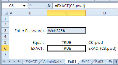
Yesterday we started the 30XL30D challenge with the action-packed, fun-filled, EXACT function. It had several examples and ways to apply it in your own workbooks.
Today we’ll investigate the AREAS function, and it’s a bit lighter in the usefulness department (to put it politely). It’s like the lazy brother-in-law, in a bad sitcom, who lies on your couch, and drinks your beer.
But, even a layabout can have a purpose. That lazy brother-in-law can serve as an example for your children, of how NOT to behave. As for the AREAS function, we can use it to see how the 3 different reference operators work, and how they affect the formula results.
So, let’s take a look at the AREAS information and examples, and if you have other examples, please share them in the comments. But don’t send me your brother-in-law!
The AREAS function returns the number of areas in a reference — an area is a range of contiguous cells or a single cell. The cells can be empty, or contain data – that has no effect on the count.

The AREAS function doesn’t have many real-world uses, but it’s an interesting example of how the reference operators work. You can use the AREAS function to do the following:
The AREAS function has the following syntax:
When entering references, you can use any of the 3 reference operators:
| : | colon | A1:B4 | Range | all cells between, and including, the two references |
| , | comma | A1, B2 | Union | combine multiple references into one |
| space | A1 B3 | Intersection | cells common to the references |
If you are using a comma in the AREAS function, to refer to multiple ranges or cells, add another set of parentheses.
=AREAS((F2,G2:H2))
Otherwise, the comma will be interpreted as a field separator, and you’ll get a “too many arguments” error.

You can use the AREAS function with a simple range reference, and the count will be 1.
=AREAS(G2:H2)

You can use the AREAS function with multiple references, to get a total count of areas. Because a comma is used as the union operator, you’ll need to add an extra set of parentheses in the formula.
=AREAS((F2,G2:H2))
The two ranges in the reference are adjacent, but are counted as separate areas, so the formula result is 2.

Even if the references overlap, or one reference is completely within another, when using the comma as the union operator, each area will be counted separately.
=AREAS((F2,F2:H2))
The two references overlap, and F2 is completely within the F2:H2 range, but they are counted as separate areas, so the formula result is 2.

When you use the space character to create an intersection from the references, the intersection areas will be counted.
=AREAS(TESTREF01 TESTREF02)
The named range TESTREF01 is coloured blue and TESTREF02 is coloured purple. These ranges intersect at three points, outlined with bold borders, so the formula result is 3.

The INDEX function, in Reference form, can use area number as its final argument.
INDEX(reference,row_num,column_num,area_num)
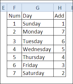
This example, based on an Excel newsgroup post by Leo Heuser, refers to a non-contiguous named range – TestBlock.
In the INDEX formula, TestBlock is the reference, and the AREAS function calculates the number of areas in the TestBlock range.
To get the value from TestBlock, row 5, column 1, last area, use this formula:
=INDEX(TestBlock,5,1,AREAS(TestBlock))
The last area is Day04, and the 5th value in Day04 is H05, which is the formula result.

To see the formulas used in today’s demo, you can download the AREAS function sample workbook. The file is zipped, and is in Excel 2007 file format.
Try to use each function in your own workbooks. Then, for extra brain-sticking power, teach a friend or co-worker how to use each function. When you explain it to someone else, you’ll remember it better.
To see a demonstration of the examples in the AREAS function sample workbook, you can watch this Excel video tutorial.
_____________
Welcome to the Contextures 30 Excel Functions in 30 Days (30XL30D) challenge. Thanks for voting for your favourite functions, and we will cover the top 30 Excel functions (based on total votes), from the following categories:
Continue reading “30 Excel Functions in 30 Days: 01 – EXACT”
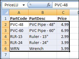
Do vampires prefer a specific blood type? Type A? Type B? Type AB? Are you positive? During the holidays, they might drink glögg, or Cosmopolitans!
Anyway, Marsha probably isn’t a vampire, but she wants to choose A or AB when doing a VLOOKUP. Here’s how you can combine values for Excel VLOOKUP formulas.
 Your great suggestions in the Improve Your Excel Skills comments got me thinking. What skills would I like to improve in 2011?
It’s hard to pick just one thing, but I’ll start with Excel functions. Even the functions that you use every day can have hidden talents, and pitfalls that you aren’t aware of. And there are so many functions, that you probably only use a fraction of them.
So, in January, let’s explore 30 Excel functions in 30 days. Yes, you’re right — there are 31 days in January. However, I’m being kind, and will give you the first day off, to recover from your hangover, and/or post-holiday exhaustion. 😉
For this challenge, we’ll stick to functions in the Text, Information and Lookup and Reference functions, listed below.
There are about 60 functions in the list, and we can only cover 30, so please vote for your favourites. If you can’t see the list below, click here to go to the form.
Deadline for voting is Wednesday, December 29, 2010, at 5 PM (Toronto time).
We’ll start the challenge on January 2nd, and go till January 31st. Please check the blog every day during the challenge, and add your tips and comments, or even a HYPERLINK. There’s no SUBSTITUTE for team work, to ensure we ADDRESS all AREAS of each function.
My mind ISBLANK now, and I can’t FIND any more puns, so I’ll sign off now, and let you CHOOSE your functions. Thanks!
Update: Thanks for voting before the December 29th deadline — votes are no longer being accepted.
___________