
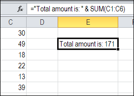
It’s easy to add a line break when you’re typing in an Excel worksheet. Just click where you want the line break, and press Alt + Enter. But how can you add a line break in an Excel formula?
Category: Excel Formulas
Excel Function Friday: Average Top 10 Scores
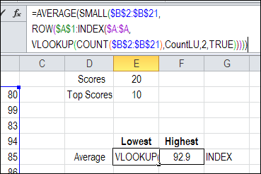
If you have a worksheet with 20 scores listed, how can you calculate an average top 10 scores? And if there are only 11 scores, can the formula automatically adjust, to average just the top 4 scores?
Continue reading “Excel Function Friday: Average Top 10 Scores”
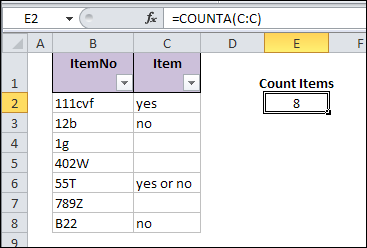
How to Find MIN IF or MAX IF in Excel
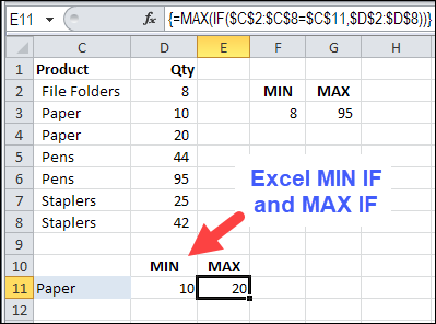
When you were first learning how to use Excel, you quickly discovered the basic Excel functions, like SUM, COUNT, MIN, MAX, and AVERAGE. Now you’re ready for advanced calculations, like how to find MIN IF or MAX IF in Excel.
Excel CONVERT Function Made Easy
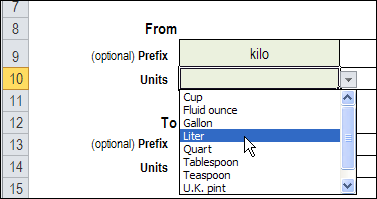
Do you ever use the Excel CONVERT function? Or, do you avoid that function, because you can’t remember all the measurement unit codes?
For example, the formula =CONVERT(10,”klt”,”gal”) will convert 10 kilolitres to 2,641.7205 gallons – if you get those codes right.
You might be able to remember lt and gal, but probably not many of the other codes.
Find Best Price With Excel INDEX and MATCH
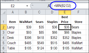
If you’re setting up a new office, or going grocery shopping, you can use Excel to compare prices. Find best price with Excel INDEX and MATCH functions, combined with MIN. This will help you calculate the lowest price for each item, and see which store sells at that price. Then, print a list, and go shopping!
Continue reading “Find Best Price With Excel INDEX and MATCH”
Troubleshoot Excel With Formula View
If you’re working in Excel, there are times when things don’t go right, and you have to do a bit (or a lot!) of troubleshooting.
Lets look at a couple of quick ways to troubleshoot Excel with Formula view, to see the worksheet formulas, and a simple trick for seeing both the formulas and the results.
Fix Blank Excel Cells Copied From Database
When you copy data to Excel, from another application, blank cells in the data can cause problems. Everything looks okay, at first glance, but the database blank cells don’t behave like other blank cells in the workbook. See how to fix blank Excel cells copied from a database, or created within Excel.
Continue reading “Fix Blank Excel Cells Copied From Database”
Excel Function Friday: Track Driver Hours
Thanks for your formula suggestions on Wednesday’s blog post about promotional pricing.
Here’s another formula example, and I’m sure you’ll have alternate methods for this problem too.
Driver Limits
In some countries, there are limits to the hours that truck drivers can work in a string of consecutive days.
In this example, the limit is 60 hours, in any period of 7 consecutive days.
Worksheet Entry Cells
The maximum hours is entered in cell C1, and the number of consecutive days is entered in cell F1.
If the regulations change, it will be easy to change those settings.

Calculate Remaining Hours
To help prevent drivers from going over their limits, we’ll set up a table where the daily hours are entered.
The date and driver name are entered in each row, in columns B and C.
In column D, the following SUMPRODUCT formula calculates how many hours the driver has remaining, in the current 7 day period.
=$C$1-(SUMPRODUCT(--($B$4:$B4>=$B4-F$1-1), --($C$4:$C4=$C4), --($E$4:$E4))-E4)
The SUMPRODUCT formula checks all the rows above the formula’s row, where:
- the date within the 7 day range
- the driver name matches the name in the current row.
That amount is subtracted from the maximum hours allowed.

Calculate the Consecutive Hours
The current hours are typed in column E, and a simple formula in column F calculates the total for a consecutive 7 day period.
=$C$1-D4+E4

Highlight the Violations
With Conditional Formatting, you can highlight any cells where the total consecutive hours exceeds the maximum allowed.
- On the Ribbon’s Home tab, click Conditional Formatting
- Click Highlight Cells Rules, and then click Greater Than

- In the Greater Than dialog box, select cell C1 as the limit in the text box.
- Select one of the preset format, or create a custom format to highlight the cells.

View the Results
With the conditional formatting applied, it’s easy to see where the trouble is.
In this example, Lou has gone over the limit on April 10th.

Download the Driver Limit Sample File
To see the data and the formulas, you can download the Driver Hours Limit sample file. The file is zipped, and is in Excel 2003 format.
There is also a pivot table that totals the drivers’ hours per calendar week.
__________
Excel Price Lookup: VLOOKUP or INDEX
This week, Glen emailed me for advice on extracting prices from a lookup table. Some products have a promotional price each month, but other products are sold at the regular price.
Pricing Lookup Table
I’m blocking email attachments these days, so I can’t show you the exact setup of Glen’s Excel worksheet.
However, a simplified version might look something like this:

Use VLOOKUP to Find Pricing
In his email, Glen mentioned that he is using a VLOOKUP formula.
- If there is a promotional price, he wants VLOOKUP to return the value from the Promo Price column.
- If there is no promotional price, Glen wants the price from the Regular Price column.
Use IF Function
To do that, Glen could use the IF function, with VLOOKUP:
=IF(VLOOKUP(F3,$B$3:$D$6,2,0)=0,
VLOOKUP(F3,$B$3:$D$6,3,0),
VLOOKUP(F3,$B$3:$D$6,2,0))

CHOOSE the Right Price
Another option is to use the MATCH function to find the row that the product is in.
In the screen shot below, the following formula is in cell H3:
=MATCH(F3,$B$3:$B$6,0)

CHOOSE and INDEX Functions
Next, in cell G3, use the CHOOSE function and the INDEX function, to get the correct price:
=INDEX(CHOOSE((INDEX($C$3:$C$6,H3)>0)+1,
$D$3:$D$6,$C$3:$C$6),H3)

How the CHOOSE Formula Works
In this example, the CHOOSE function selects the correct pricing column to use for the prices. The outer INDEX function returns the price from the selected column.
First, the inner INDEX function returns the price from the promo column, for the selected product, and we check to see if the price is greater than zero:
INDEX($C$3:$C$6,H3)>0
- If there is NO promo price, the result is FALSE (0)
- If there IS a promo price, the result is TRUE (1)
Next, we add 1 to that result, so
- FALSE=1
- TRUE=2.
CHOOSE the Range
Next, the CHOOSE function returns a reference to the selected range.
- FALSE (1) = $D$3:$D$6
- TRUE (2) = $C$3:$C$6
Finally, the first INDEX function returns a price from the selected column, in the row for the selected product.
How Would You Solve the Problem?
I’m sure there are several other ways to solve Glen’s lookup problem. What formula would you use?
________________
Excel Function Friday: Subtotal and Sumproduct with Filter
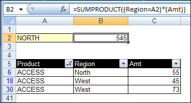
Last week, we used the Excel SUBTOTAL function to sum items in a filtered list, while ignoring the hidden rows. Now we’ll look at ways to use Subtotal and SumProduct with filter settings applied.
Continue reading “Excel Function Friday: Subtotal and Sumproduct with Filter”