We looked at the Excel SUBTOTAL function on Friday, and saw how it works with hidden rows.
- The first argument tells Excel which function you want to use, such as SUM (9), MAX (4) or AVERAGE (1).
Excel tips and tutorials

We looked at the Excel SUBTOTAL function on Friday, and saw how it works with hidden rows.
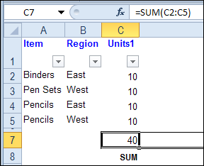
The Excel SUM function does a great job of adding numbers on a worksheet, and it’s probably the first Excel function that you learned about.
But SUM might not be the best function to use in all situations where you need a total.
Continue reading “Excel Function Friday: Sum Filtered List With SUBTOTAL”
ISREF and the IS Functions — although it sounds like the name of a geeky band, it’s not. Today we’ll take a look at ISREF, which is one of the 9 IS functions that are lumped together in the Excel Help files.
How sad — 9 functions that never get to shine on their own. We’ll give ISREF a few minutes in the spotlight, to see how it works.
The following IS functions are listed on one page in Excel Help:
They all work in the same way — the function tests a value, and returns TRUE if the value passes the test.
NOTE: There is also a new ISFORMULA function for Excel 2013 and later versions.
For example, if cell B2 contains a number, the ISNUMBER formula will result in TRUE:
=ISNUMBER(B2)

If cell B3 contains anything except text, even if cell B3 is blank, the ISNONTEXT formula will result in TRUE:
=ISNONTEXT(B3)

The other IS functions work the same way, and give the expected results — except for ISREF.
In the screen shot below, there is a reference in cell B2, with the following formula: =D1
In cell D2, the ISREF function returns TRUE as the result.
However, the ISREF function also returns TRUE in cell D3, even though there is a typed value in cell B3 — the number 7

The ISREF function isn’t testing what’s in the referenced cell, it’s testing the reference within the formula.
And because the ISREF formulas in both D2 and D3 contain references, the result is TRUE for both formulas.
So, the ISREF function won’t help you assess whether there is a reference another cell.
If you can’t use ISREF to detect a reference in another cell, how can you use it?
Well, ISREF can check the results of other formulas, to see if they have returned a valid reference.
You could use ISREF, instead of ISERROR, in your formulas that need references.
For example, in the screen shot below, the INDIRECT function in cell D2 returns a reference, and INDIRECT(“D1”) creates a valid reference.
If cell B2 contains the text “D1”, this formula results in TRUE:
=ISREF(INDIRECT(B2))

The first OFFSET formula in the screen shot below is not valid, because there is no cell that is 1 column to the left of cell A1, so the ISREF result is FALSE
=ISREF(OFFSET(A1,0,-1))
Hoever, the second OFFSET formulas returns a valid reference to cell B1, so the ISREF result is TRUE.

Do you use ISREF in your formulas? Can you think of any other examples for using it?
______________
Last Friday, there was an HLOOKUP example, and it used a dynamic lookup range — as rates were added to the lookup table, it automatically expanded to include them.
Continue reading “Excel Function Friday: INDEX for Dynamic Range”
 On Day 10 of the 30 Excel Functions in 30 Days series, we looked at the Excel HLOOKUP function. It’s similar to VLOOKUP, but looks for values in a horizontal list, instead of a vertical list.
The second example in that HLOOKUP blog post showed how to find a rate in a lookup table, based on the date entered in cell C5. On March 15th, the rate would be 0.25, because the Jan 1st rate is still in effect.

In the comments for the HLOOKUP blog post, Fred said that he got the formula working correctly in cell D5, but wondered how to use the result in multiple cells.
In this example, we’ll use the rates as a lookup for pricing. The prices change quarterly, and the correct price will be used in each order, based on the order date.

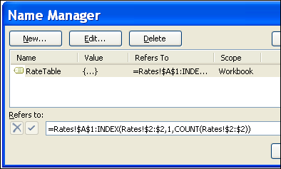
In this workbook, the table with the quarterly dates and rates is on a separate sheet, named Rates.
New rates will be added each quarter, so we’ll create a dynamic range named RateTable, using the technique from Example 3 in the 30XL30D INDEX function post.
In this HLOOKUP rates table, the formula for the named range is:
=Rates!$A$1:INDEX(Rates!$2:$2,1,COUNT(Rates!$2:$2))

In the Orders table, we’ll use an Excel HLOOKUP formula to pull the correct rate from the RateTable range, based on the order date.
In cell B2, the formula is:
=HLOOKUP(A2,RateTable,2)
The final argument is omitted, so the result is an approximate match.
If the order date isn’t found in the first row of the RateTable range, the HLOOKUP formula result is based on the next largest date that is less than order date.

The final step is to add the pricing formula in column D. Quantities will be entered in column C, so the pricing formula will multiply the quantity by the rate.
The formula in cell D2 is:
=B2*C2
To see the Excel HLOOKUP formula and the RateTable named range, you can download the HLOOKUP Rates sample file.
It is in Excel xlsx format, and zipped.
_______________
 Yes, it’s Valentine’s Day today, and if you were too busy to buy your sweetie a card yesterday, you can make one in Excel. Phew!
Your boss won’t mind if you spend a couple of hours working on this today, because it’s an Excel project! This Excel Valentine card uses a named range, data validation, a formula, and conditional formatting (to change the heart from white to pink to red).
If you won’t have time, or if your drawing skills are worse than mine, you can download the sample Excel Valentine file, at the end of this blog post.
And if you want some romantic music in the background, while you work on your Excel Valentine card, you can listen to the YouTube playlist, compiled by John Walkenbach and his blog readers.
To create the heart shape,

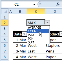
The formula will count how many text items have been added at the top of the worksheet, and the result is used for conditional formatting.
=COUNTA($E$1:$E$3)

With the Heart range still selected, set up the following conditional formatting:

The heart shape will be hidden, and only revealed when the Valentine message is selected.
To hide the heart:
Next, you’ll create three drop downs, for the Valentine message at the top of the worksheet.
To prepare the cells for the drop down lists:

Create the following data validation drop down lists:
Tip: To type a heart shape, press Alt and type a 3 on the number keypad (if no number keypad, try Fn+Alt+L). On a Mac, another key combination might be needed.

The Excel Valentine heart has white fill and white font, so it’s not visible.
To see the heart:

To see how the card works, you can download the Excel Valentine Card sample file.
The file is in Excel 2007 format, and zipped, and it contains no macros.
_____________
Apparently there is a big football game this weekend in the USA. They’re using Excel for the game — XLV. That’s a really old version, but at least it has multiple sheets and VBA!
The officials probably used the Excel ROMAN function to figure out how to show the game number — 45:
=ROMAN(A2)

While you’re watching the game, you can use an Excel function to convert the field size from yards to metres. You’ll see that the American field is smaller than the Canadian field, no matter what measurement system you use!
There is a CONVERT function in Excel, that you can use to convert measurements from one system to another.
=CONVERT(number,from_unit,to_unit)
For example, cell B3 has the length of a Canadian field in metres. In cell D3, the following formula converts that measurement to yards, and rounds the result:
=ROUND(CONVERT(B3,B$2,D$2),0)

Unfortunately, the CONVERT function does not get you an extra point.
Besides the size of the fields, there are other key differences between Canadian and American football.

No stripes? Fewer players? More downs? You call that a game? 😉


Do you remember when printed manuals came with the software? I still have my Excel 5.0 User Guide, so maybe I can read it while watching the big game!
There were tons of new features in that version, so there will be lots of interesting stuff to read.

________________
Thanks for participating in the 30XL30D challenge, that ended yesterday.
My favourite Excel function in the series was INDEX — I learned a few useful tricks while researching that one! How about you?
Continue reading “30 Excel Functions in 30 Days: Conclusion”
 Congratulations! You made it to the final day in the 30XL30D challenge. It’s been an long, and interesting, journey, and I hope you learned a few useful things about Excel functions along the way.
Tomorrow, I’ll do a wrap-up article, and let you know how the functions ranked in the pre-challenge voting, last month.
For day 30, we’ll examine the INDIRECT function, which returns the reference specified by a text string.
This is one of the ways that you can create a dependent data validation drop down list, where, for example, the selection in the Country drop down controls the choices in the City drop down.
So, let’s take a look at the INDIRECT information and examples, and if you have other tips or examples, please share them in the comments.
The INDIRECT function returns the reference specified by a text string.

The INDIRECT function returns the reference specified by a text string, so you can use it to:
The INDIRECT function has the following syntax:
In the first example, there are identical numbers in columns C and E, and the totals are the same, using the SUM function. However, the formulas are slightly different. In cell C8, the formula is:
=SUM(C2:C7)
In cell E8, the INDIRECT function creates a reference to the starting cell, E2:
=SUM(INDIRECT(“E2”):E7)

If a row is inserted at the top of the lists, and January amounts are entered, the total in column C doesn’t change. The formula changed, adjusting to the inserted row:
=SUM(C3:C8)
However, the INDIRECT function locked the starting cell to E2, so the January amount is automatically included in the column E total. The ending cell changed, but the starting cell wasn’t affected.
=SUM(INDIRECT(“E2”):E8)

The INDIRECT function can also create a reference for a named range. In this example, the blue cells are in a range named NumList. There is also a dynamic range in column B, based on the count of numbers in that column.
The total for either range can be calculated, by using the range name with the SUM function, as you can see in cells E3 and E4
=SUM(NumList) or =SUM(NumListDyn)

Instead of typing the name in the SUM formula, you can refer to the range name in a worksheet cell. For example, with the name NumList in cell D7, the formula in cell E7 is:
=SUM(INDIRECT(D7))
Unfortunately, the INDIRECT function can’t resolve a dynamic range, so when the formula is copied down to cell E8, the result is a #REF! error.

You can easily create a reference based on row and column numbers, by using FALSE as the second argument in the INDIRECT function.
This creates an R1C1 style reference, and in this example, a sheet name is also included — ‘MyLinks’!R2C2
=INDIRECT(“‘” & B3 & “‘!R” & C3 & “C” & D3,FALSE)

In some formulas, you need an array of numbers, as in this example, where we want the average of the 3 highest numbers in column B. The numbers could be typed in the formula, as they are in cell D4:
=AVERAGE(LARGE(B1:B8,{1,2,3}))
If you need a bigger array of numbers, you probably wouldn’t want to type all of them. Another option is to use the ROW function, as in the array-entered formula in cell D5:
=AVERAGE(LARGE(B1:B8,ROW(1:3)))
A third option is to use the ROW function with INDIRECT, as in the formula in cell D6, which is also array-entered:
=AVERAGE(LARGE(B1:B8,ROW(INDIRECT(“1:3”))))
The results for all 3 formulas are the same.

However, if rows are inserted at the top of the sheet, the second formula returns an incorrect result, because the rows are adjusted. Now, instead of the average of the top 3 numbers, it shows the average of the 3rd, 4th and 5th largest numbers.
With the INDIRECT function, the third formula keeps the correct row reference, and continues to show the correct result.

To see the formulas used in today’s examples, you can download the INDIRECT function sample workbook.
The file is zipped, and is in Excel 2007 file format.
To see a demonstration of the examples in the INDIRECT function sample workbook, you can watch this short Excel video tutorial.
_____________
Yesterday, in the 30XL30D challenge, we jumped around a workbook, and opened Excel files and websites, by using the HYPERLINK function.
For day 29 in the challenge, we’ll examine the CLEAN function. Sometimes the data you get from a website, or in a download file, has some unwanted characters, and the CLEAN function can help you fix it.
It doesn’t do much heavy lifting though, and refuses to help with the mess that the kids make. This will be perfect for a lazy Sunday!
So, let’s take a look at the CLEAN information and examples, and if you have other tips or examples, please share them in the comments.
The CLEAN function shows removes some non-printing characters from text — characters 0 to 31, 129, 141, 143, 144, and 157.

The CLEAN function can remove some non-printing characters from text , but not all of them. You can use CLEAN, or other functions when necessary, to:
The CLEAN function has the following syntax:
The CLEAN function only removes some non-printing characters from text — characters 0 to 31, 129, 141, 143, 144, and 157.
For other non-printing characters, such as the non-breaking space character 160, you can use SUBSTITUTE to replace them with space characters, or empty strings.
The CLEAN function works to remove some non-printing characters, such as those in the 0-30 range of the ASCII character set. In this example, I added characters 9 and 13 to the original text string from C3.
=CHAR(9) & C3 & CHAR(13)
The LEN function shows that the number of characters in cell C5 increased to 15, with those non-printing characters included.

With the CLEAN function, in cell C7, those characters are removed, and the number of characters is reduced by 2, so it’s back to the original 13 characters.
=CLEAN(C5)

For the characters that the CLEAN function can’t remove, like characters 127 and 160, you can use the SUBSTITUTE function to replace them.
=SUBSTITUTE(E3,CHAR(C3),””)

To see the formulas used in today’s examples, you can download the CLEAN function sample workbook. The file is zipped, and is in Excel 2007 file format.
To see a demonstration of the examples in the CLEAN function sample workbook, you can watch this short Excel video tutorial.
_____________