
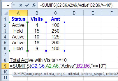
In Excel 2007 and Excel 2010, you can use the new SUMIFS function to sum items using multiple criteria.
Category: Excel Formulas
Use Excel COUNTIFS to Count With Multiple Criteria
In Excel 2007 and Excel 2010, you can use the new COUNTIFS function to count, based on multiple criteria.
For example, in a list of orders, you can find out how many orders were for pens, and had a quantity of 10 or more.

Page Updates
I have updated the Contextures COUNT Functions page, to include a COUNTIFS example, and video demo.
If you are using Excel 2003, or earlier versions, you can use the SUMPRODUCT function instead. There is an example for that function on the COUNT page too.
Watch the COUNTIFS Video
To see the steps for using the COUNTIFS function, you can watch this short Excel video tutorial. The written steps are on the Contextures COUNT Functions page.
There is a complete transcript of the tutorial directly beneath the video.
VIDEO TRANSCRIPT
Counting With Criteria
In Excel you can count using criteria with the COUNTIF function.
In later versions of Excel (2007 and later) you can count multiple criteria with the COUNTIFS function.
So here we have a list of items that we’ve sold and the quantity for each.
We would like to find the number of orders where a pen was the item sold and the quantity is greater than 10.
First Criteria
So in this cell I’m going to start with an equal sign and then type COUNTIFS an open bracket and the first thing I’m going to check is the item that was sold.
The range, first range is A2:A10. Then I’ll type a comma and the criteria for that range I’m just going to type in here inside double quotes pen, and then another comma.
That’s the first thing we’re going to check, is what item was sold.
Additional Criteria
Next will be the quantity so I’ll select the range that has the quantities, another comma and we want quantity greater than or equal to 10 so within double quotes
I’ll do a greater than symbol, equal, and a 10, then another double quote
Close the bracket and press Enter. There were two orders for pen where the quantity is greater than 10. Instead of typing these criteria in here I can refer to a cell.
So instead of typing pen inside double quotes, I could click on a cell where I have typed the word pen. The same for this criteria for the quantity
I’m going to take out the 10 just by deleting that, leaving the operators within the double quotes.
Adjustments
Then I’ll type an ampersand and the cell that has the number. So this is greater than or equal to whatever number is in cell E3.
When I press ENTER I get the same result. It’s just easier to change.
Then I could type a 5 here now, and we see that there were 4 orders where the quantity is greater than or equal to 5 instead of the 10 that we had in there before.
So this formula is much more flexible if you use cell references, rather than typing the values in as hard-coded values.
End Of Transcript
_________
Excel VLOOKUP Troubleshooting
You’re admired by your co-workers, thanks to your awesome Excel skills. Cupcakes magically appear on your desk, in thanks for your help with complex formulas.
Your boss keeps stretching the budget, to accommodate the huge bonuses you get, in reward for your amazing talents. Well, that might not be the exact situation, but I’m sure your skills are appreciated!
VLOOKUP Trouble
Then, one day, it all goes horribly wrong. Your boss needs a report in 15 minutes, and you can’t get a seemingly simple VLOOKUP formula to work.
You can see the target product numbers in the lookup table, but the formula result is #N/A, instead of the product price.

You don’t want to lose your Excel Expert badge over something this trivial, so how will you solve the problem?
Text or Number?
A common cause for this VLOOKUP error is that one of the values is a number, and the other is text. In this example, the lookup table codes in cell B2:B5 are stored as text values – they have a leading apostrophe.
The lookup code, in cell B8, is entered as a number – no leading apostrophe.

So, it looks like cells B2 and B8 are equal, but Excel sees them as different values.

Fix the Text Values
The easiest solution to the the VLOOKUP problem in this example is to convert the text values to numbers, so the codes in the table match your lookup values.
Or, type an apostrophe in front of your lookup code in cell B8, so it’s a text value too.
Change the VLOOKUP Formula
If you can’t fix the data, you can convert the lookup value in the Excel VLOOKUP formula. Here is the original VLOOKUP formula, that returned an #N/A error.
=VLOOKUP(B8,$B$2:$D$5,2,FALSE)
If you add an empty string to the end of the value in cell B8, the lookup number will be converted to a text string. The revised formula is:
=VLOOKUP(B8 & “”,$B$2:$D$5,2,FALSE)
This formula will also work if cell B8 contains a text value – adding the empty string won’t change the value.
More Excel VLOOKUP Troubleshooting
If this VLOOKUP formula fix doesn’t solve the problem, there are more Excel VLOOKUP troubleshooting tips on the Contextures website.
Have you run into this problem? How did you fix it?
Watch the Excel VLOOKUP Troubleshooting Video
To see the steps for fixing the Excel VLOOKUP problem, you can watch this short Excel video tutorial.
___________________
Calculate Thanksgiving Date in Excel
Recently, Jerry Latham showed us how to use Excel to calculate the date of Easter in any year, by using a worksheet formula or Excel User Defined Function (UDF). Now, it’s getting close to Thanksgiving in the USA, so lets see how to calculate that date, with an Excel worksheet formula.
Words to Numbers in Excel
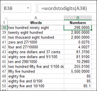
There are Excel formulas and User Defined Functions (UDF) that can change numbers into words. Those are handy if you’re typing a number into a workbook, and want the written amount to be shown, as it might appear in a cheque. Have you ever tried to do the opposite – change words to numbers in Excel?
Create Random Scenarios in Excel
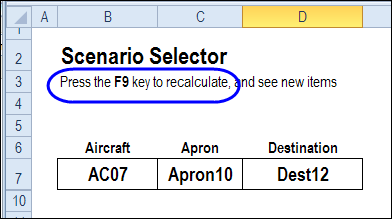
My son is in an Air Traffic Control course, and there’s lots of information to memorize. Directions have to be given in a very specific sequence, or the pilots don’t respond. Apparently, you can’t say, “Hey dude, just put it down anywhere.” No, you have to address the aircraft correctly, and specify an apron and refer to a valid destination. Or something like that!
Continue reading “Create Random Scenarios in Excel”
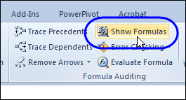
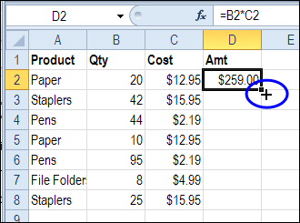
Excel Formulas Show in Cell
Last year, I showed that you could combine text in Excel by using the ampersand (&) operator, instead of the CONCATENATE function. That makes it much easier for those of us who are lazy, or can’t remember how to spell concatenate.
Quickly Copy Excel Formula Down
You probably know how to quickly copy Excel formula down a column, if there is data in the next column. But how can you do the same thing, if there are blank rows?
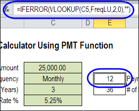
Change Excel Formula Results With CheckBox
You spent hours creating an impressive table of loan payment calculations. Different loan amounts are across the top of the table, and a variety of terms and interest rates are at the left side.
At a glance, you can see the monthly payment for any combination of variables. Sweet!

Then, your boss breaks your magical spell of awesomeness, by asking you to include the total payments for each combination.
Sure, you could copy that sheet, and tweak the formulas, or add more columns, but then the workbook is
- double the size, and
- twice the maintenance.
Use a CheckBox
Thanks to Dave Peterson, there’s a new tutorial and sample file on the Contextures website – Excel Formula CheckBox. Instead of duplicating your work, and creating multiple sheets, you can solve the problem with a simple checkbox.
A checkbox at the top of the worksheet is linked to cell C1. If the box is checked, C1 is TRUE, and if it’s not checked, C1 is FALSE.
The loan payment formulas are modified, to include a reference to cell C1. The the box is checked, the monthly payment is multiplied by the total number of payments. The loan payment table shows the total amount to be repaid, instead of the monthly payment.

Other Uses for CheckBox Formulas
Of course, this technique isn’t limited to loan payment tables. You can use a checkbox selector in other workbooks too — for example, let users specify if tax should be included, or check the box if they want to see prices converted to US dollars.
Do you have any other ideas for changing the formula results with a checkbox?
Download the Sample File
For the detailed instructions, please visit the Contextures website – Excel Formula CheckBox. You can download the sample file there too.
___________
Excel Loan Payment Calculator
Can you afford that new car? Or maybe you loaned money to one of your kids, and you want to calculate a repayment schedule. (Oh yes, they will stick to the plan, without fail.)
To help you figure out the payment amounts, here is a nifty Excel loan payment calculator. (The kids will think you’re cool when you say “nifty”.)