Highlight Duplicate Records in an Excel List

With Excel’s conditional formatting, you can highlight cells based on specific rules. There are some built-in rules available, and you can use formulas to create your own formatting rules.

Highlight Duplicates

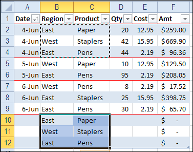
In this example, we want highlight duplicate records in a table. There is a built-in rule for highlighting duplicate values in a single column, but nothing that will check an entire row.

built-in rule for highlighting duplicate values

So, we’ll create our own rule, and it will require a new column on the worksheet, before we add the conditional formatting.

Concatenate the Data

In the sample data, there are two identical rows, and these should be highlighted after we apply our conditional formatting.

two identical rows in sample data

The first step is to use the CONCATENATE function to combine all the data into one cell in each row.

Add a new heading in cell G1 – AllData – and in cell G2, enter this formula, to combine the data from all the cells in that row.

=CONCATENATE(A2,B2,C2,D2,E2,F2)

formula to combine the data

Next, copy the formula down to the last row of data.

Apply the Conditional Formatting

Then, a conditional formatting rule is set, to color the rows that are duplicate records. We’ll use the COUNTIF function to check for duplicates in the AllData column.

=COUNTIF($G$2:$G$8,$G2)>1

create new conditional formatting rule

If there is more than one instance of a data combination, that indicates a duplicate row, and the cells in columns A:F will be coloured. The two rows with duplicate records are highlighted, so our conditional formatting formula worked!

duplicate records are highlighted

Download the Sample File

For detailed instructions, and to download the sample file, please visit my Contextures website: Highlight Duplicate Records in a List

Watch the Video

To see the steps for setting up the conditional formatting, watch this short video.

_________________________

Format Excel Worksheet for Troubleshooting

Do you ever get sent an Excel file, and asked to figure out why it’s not working correctly? The odds are that it was created several years ago, by someone who has left the company, and a few other people have “improved” it over the years.

Now it’s a mess, and nobody is sure exactly how it works. It’s up to you to sort it out. Lucky you!

Here’s how I start the troubleshooting process, and you can see the steps in the video below. There are detailed instructions on my Contextures site.

Make a Copy of the Original File

In the screen shot below, you can see a worksheet that is similar to the ones that I troubleshoot. There is a rainbow of colours on the sheet, but they don’t seem to have any significance – they’re just someone’s favourite colours.

I’ll get rid of that rainbow, and colour the cells that contain:

  • formulas
  • text
  • numbers
  • data validation

But the first step is to make a copy (or two) of the original file, and store it in a safe place. Don’t make any changes to the file, until you have that backup file safely stored away – you might want to refer to it later, as you dig deeper into the troubleshooting.

Price Calculation Sheet with coloured cells

Clear All Colour

The next step is to remove all the colour fill from the worksheet, so you can add your own colour scheme.

  1. Select all the cells on the worksheet
  2. Choose No Fill as the cell fill colour

When you’re finished troubleshooting, and the worksheet is functioning correctly, you can clear the troubleshooting formats.

Then, add colour to the data entry cells, or other key cells, to help people understand how the workbook should be used.

Colour the Formula Cells

The next step is to find and format the cells that contain formulas.

  • On the Ribbon’s Home tab, click the Find & Select command
  • Click on Formulas, to select all the formula cells

Find Formulas

  • Then, use the Fill command on the Ribbon to format the Formula cells. I usually use grey for the formula cells, which indicates that they shouldn’t be changed.

Colour Remaining Cells

Next, you can find and format the cells that contain constants, and data validation, by using the other options in the Find & Select drop down.

  1. On the Ribbon’s Home tab, click the Find & Select command
  2. Click on Constants, then format the Constant cells.
  3. Repeat the steps to format the Data Validation cells, where drop down lists or special rules apply

Colour Constant Numbers

Finally, find and format the cells that contain constant numbers. These might be data entry cells, that you can use in testing the worksheet.

  • On the Ribbon’s Home tab, click the Find & Select command
  • Click the Go To Special command.
  • Select Constants, and check the box for Numbers. Remove the check mark in the Text, Logicals and Errors boxes, then click OK.

Go To Special dialog box

  • Then, format the constant number cells

Finish Worksheet Formatting

After all the key cells are colour coded, you can add a legend on the worksheet, to show what the colours mean.

Then, get started with the troubleshooting. For example, in the screen shot below, the circled cells contain constants, but they should contain formulas.

get started with worksheet troubleshooting

Watch the Formatting Video

To see the steps for formatting the different types of cells, you can watch this short video.

___________________

Line Between Dates in Filtered List

A while ago, I showed you how to add a red border at the top of a row, when a new date starts in a list.

You can read those instructions here: Separate Excel List with Automatic Lines.

Line Between Dates in Filtered List

Conditional Formatting Problem

And if you’re using this technique, remember the painful lesson that I learned – don’t copy and paste within a table that has conditional formatting.

You could end up with an Excel 2010 Conditional Formatting Nightmare. And nobody wants that!

conditional formatting duplicate rules problem

Lines Disappear in Filtered Lists

Recently, I heard from Lon, who liked the tip about red line borders. But Lon noticed a problem – the line didn’t always show if the list was filtered.

For example, if we filter the Product column, to hide Paper, the red borders for some of the dates disappear.

Lines Disappear in Filtered Lists

I hadn’t noticed the problem, because my list is usually filtered by date, to show only the latest month’s data. Since the conditional formatting is based on the date column, it would continue to work correctly.

But we can change the conditional formatting, so it works in a filtered list.

Change the Formula for Filtered Lists

To make the conditional formatting work in a filtered list, we can’t use the original formula, which was

=$A1<>$A2

That formula just compares each date to the date above it, and doesn’t care if the rows are hidden or visible.

Instead, we’ll use a formula that was created by Laurent Longre. It lets you work with visible rows after a filter. For information on this formulas, read the Power Formula Technique section, in this article at John Walkenbach’s web site: Excel Experts E-letter

Here is the much longer formula that we can use, to compare dates in the visible rows only.

=SUMPRODUCT(SUBTOTAL(103,OFFSET($A$1:$A2,ROW($A$1:$A2)
-MIN(ROW($A$1:$A2)),,1)), –($A$1:$A2=$A2))=1

Note that there are two minus signs in front of the last open bracket – it’s not a long dash.

ConditionalFormatFiltered03

Date Separator Lines Show When Filtered

With the new formula, the red lines separate the dates, even if the list is filtered. In the screen shot below, the Product column is filtered to hide Paper, but the date line for July 18th shows up.

Date Separator Lines Show When Filtered

Download the Sample File

There is another example of this type of formula on my Contextures website – Count Visible Items in a Filtered List.

And you can download the sample file used in this blog from the Contextures Sample Excel Files page. In the Conditional Formatting section, look for CF0004 – Conditional Formatting in Filtered List. The zipped file is in Excel 2007/2010 format, and contains no macros.

_________________

Excel 2010 Conditional Formatting Nightmare

[Updated June 2018] I’m a big fan of Excel’s conditional formatting, and often use it to highlight cells on a worksheet. But this week I ran into a conditional formatting nightmare, and had to start from scratch. Fortunately, the fix didn’t take too long, but with complex formatting, things could have been much worse.

Continue reading “Excel 2010 Conditional Formatting Nightmare”

Separate Excel List with Automatic Lines

When you create a table in Excel, you can use the built-in styles, to add bands of colour.

ConditionalFormatSections

The colour bands can make the table easier to read, because you can follow each line across, using the colour as a visual guide.

Separate the Days in the List

If you’re working with a list of tasks or orders, sorted by date, those coloured bands don’t help you see where each day’s data starts and ends.

To make it easy to separate the days, you can add conditional formatting to the table. We’ll add a line at the start of each date, to highlight those rows.

  • Select all the cells in the body of the Excel table. In this example, cell A2 is the active cell, and A2:F9 are selected.
  • On the Ribbon’s Home tab, click Conditional Formatting, then click New Rule

ConditionalFormatSections02

  • In the New Formatting Rule dialog box, click Use a Formula
  • In the formula box, enter this formula, which compares the values in cells A1 and A2. There is a $ before each A, because we need an absolute reference to column A.
    • =$A2 <> $A1

ConditionalFormatSections05

  • Click the Format button
  • In the Format dialog box, click the Border tab
  • Select a border pattern and colour, to separate the dates. Unfortunately, you can’t select a thickness for the border line.
  • Click the top border in the preview window, and click OK

ConditionalFormatSections03

  • Click OK to close the New Formatting Rule dialog box.

There will be a border at the start of each date in the table, and you’ll see at a glance where the dates start and stop.

ConditionalFormatSections04

More Conditional Formatting Examples

You’ll find many more conditional formatting examples and tutorials on the Contextures website.

Watch the Excel Video Tutorial

To see the steps for adding lines between the dates, you can watch this short Excel video tutorial.

___________

How to Add Bullets in Excel

There’s no built-in feature for bullets in Excel, like there is in a Word document. Bullets are a handy feature when you’re making a list, so it would be nice to use them occasionally, in our Excel files. Even though they’re not built in, keep reading, to see how to add bullets in Excel.

Continue reading “How to Add Bullets in Excel”