Excel Footer with Formatted Date

It’s Fancy Footer Friday! Check with your boss – maybe you can leave early to celebrate.

This week, I’ve been working on Excel printed reports, and one of my clients wanted some fancy features in the footer. There are built-in footer options in Excel, but my client wanted to pull information from the worksheet, and format the date, so we needed some footer programming.
Continue reading “Excel Footer with Formatted Date”

Customize Excel Conditional Formatting Icons

In Excel 2007 and Excel 2010, you can use icon sets in conditional formatting. There are built-in icon sets, and in Excel 2010 you can Customize Excel Conditional Formatting Icons, to some extent. Here’s how to do that, and a workaround to create icons on the worksheet instead.

Continue reading “Customize Excel Conditional Formatting Icons”

Fix Those Wandering Excel Comments

Do you ever open an Excel workbook, and find that tragedy has struck your comments? You spent hours inserting those comments, and making them just the right size and shape. Then, for no apparent reason, everything changes. Comments are in the wrong place, and wrong size. Here’s how to fix those wandering Excel comments.

Continue reading “Fix Those Wandering Excel Comments”

Make a Valentine Card in Excel

Heart000Yes, it’s Valentine’s Day today, and if you were too busy to buy your sweetie a card yesterday, you can make one in Excel. Phew!

Your boss won’t mind if you spend a couple of hours working on this today, because it’s an Excel project! This Excel Valentine card uses a named range, data validation, a formula, and conditional formatting (to change the heart from white to pink to red).

If you won’t have time, or if your drawing skills are worse than mine, you can download the sample Excel Valentine file, at the end of this blog post.

And if you want some romantic music in the background, while you work on your Excel Valentine card, you can listen to the YouTube playlist, compiled by John Walkenbach and his blog readers.

Set Up the Worksheet

To create the heart shape,

  1. Start by making columns A:M narrower, to create square cells
  2. Then, add red fill colour to cells in rows 5:14, to create a heart shape
  3. Select the coloured cells, and name the range as Heart

Heart01

Add the Formula

The formula will count how many text items have been added at the top of the worksheet, and the result is used for conditional formatting.

  1. Select the Heart range
  2. Type the following formula, then press Ctrl+Enter, to enter the formula in all the selected cells:

=COUNTA($E$1:$E$3)

Heart02

Add Conditional Formatting

With the Heart range still selected, set up the following conditional formatting:

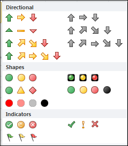
  • =1, light pink fill and font
  • =2, dark pink fill and font
  • =3, red fill and font

Heart03

Hide the Heart

The heart shape will be hidden, and only revealed when the Valentine message is selected.

To hide the heart:

  1. Select the Heart range
  2. Format the cells with white fill and font.

Add the Data Validation Drop Downs

Next, you’ll create three drop downs, for the Valentine message at the top of the worksheet.

To prepare the cells for the drop down lists:

  1. Merge cells E1:I1, E2:I2, E3:I3 (yes, merging can cause problems, but it’s allowed on Valentine’s Day)
    • Tip: After you merge E1:I1, drag the Fill Handle, to copy the formatting down to the next two rows.
    • Heart04
  2. Add a bottom border to each merged cell, with red or dark pink border colour.

Create the following data validation drop down lists:

  • E1: I, You, Everyone
  • E2: Love, Loves, ?, Heart, Hearts
  • E3: You, Me, Excel

Tip: To type a heart shape, press Alt and type a 3 on the number keypad (if no number keypad, try Fn+Alt+L). On a Mac, another key combination might be needed.

Heart05

Use the Excel Valentine

The Excel Valentine heart has white fill and white font, so it’s not visible.
To see the heart:

  1. Select one item from the drop down lists, to colour the valentine light pink
  2. Select two items from the drop down lists, to colour the valentine dark pink
  3. Select three items from the drop down lists, to colour the valentine red

Heart07

Download the Excel Valentine Card

To see how the card works, you can download the Excel Valentine Card sample file.

The file is in Excel 2007 format, and zipped, and it contains no macros.
_____________

Use Excel Scroll Bar to Trim Christmas Tree

An Excel scroll bar can be used for practical (and sometimes boring) things, like testing the effect of price changes, or adjusting a chart’s date range.

But this is the festive season, so let’s use a scroll bar for something more, well, festive!

Trim the Tree

In this example, instead of accounting and finance, you’ll see how to use an Excel scroll bar to decorate a Christmas tree, without macros.

Unfortunately, this Excel file can’t make hot chocolate or eggnog, so you’ll need to provide your own.

Useful Excel Features

It’s not just for the holiday season though — the sample file has useful features that you can adapt to other workbooks too:

  • Scroll bar lets users change a number quickly and easily
  • A text box that displays a changing message based on VLOOKUP formula
  • conditional formatting shows hidden cells when target number is reached
  • named ranges make it easy to work with specific cells
Use Excel Scroll Bar to Trim Christmas Tree

Watch the Video

To see how the Excel Christmas tree trimming scroll bar works, you can watch this short Excel video.

Excel Scroll Bar Sample File and Instructions

For instructions on creating the Excel scroll bar file, and to download the sample file, go to my Contextures website: Excel Scroll Bar Christmas Tree Example.

Copy Pivot Table Format and Values

To keep your data details confidential, you might want to send someone a copy of a pivot table, without the link back to its source data. It’s easy to copy a pivot table, and paste it as values,but it is difficult to copy pivot table format and values.

Continue reading “Copy Pivot Table Format and Values”

Conditional Formatting From Different Sheet

A nice new feature in Excel 2010 is the ability to refer to a different worksheet when creating conditional formatting and data validation. Let’s take a look at how the conditional formatting from different sheet feature works, and create a workaround for older Excel versions.

Continue reading “Conditional Formatting From Different Sheet”