Highlight Items in 2 Excel Lists-Conditional Formatting

If there are any typos in this blog post, blame my maple syrup related injury. Sunday morning, I tried to clean a few drips from the syrup jug, and ended up with a puncture wound.

Those crystallized bits are razor sharp, so don’t put your delicate typing fingers anywhere near them. Maybe it’s just a Canadian hazard!

List of Excel Files

Bravely carrying on, I was updating some files, and keeping track of the updates in Excel.

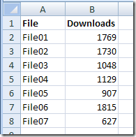
On a sheet named All_Files, I have a list of all the files, and the number of downloads for each file.
FileListAll01

On the Files_Updated sheet, I have a list of files that have been updated.
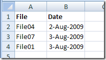
list of updated Excel files

Mark Duplicate Entries With Conditional Formatting

When looking at the full list of files, I’d like a quick way to identify the files that have been updated.

The actual list is pretty long, and my faulty memory only works for the first few updates. After that, I can’t really remember which ones have been done.

See the written steps, and an Excel video, in the sections below

Use Formula to Count Duplicates?

I could add a new column, with a COUNTIF formula to count the number of times each file appears in the Update list.

Instead, I’ll use conditional formatting to colour the rows for files that have been updated.

Highlight Duplicate Items

Just like data validation, conditional formatting complains if you try to refer to cells on another worksheet.

So, I’ll name the range on the Files_Updated sheet, and refer to the named range.

For some reason, Excel is okay with references to named ranges on another sheet.

Name the Range

To name the range:

  1. On the Files_Updated, select column A
  2. Click in the Name box, and type a one word name for the range – UpdateA in this example.
  3. Press the Enter key, to complete the naming.
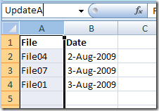
Name the Range
Name the Range

Add the Conditional Formatting

Next, add the conditional formatting to the list of all files.

  • On the All_Files sheet, select the cells that contain the file names and download quantities.
  • On the Ribbon, click the Home tab

Click Conditional Formatting, then click New Rule.
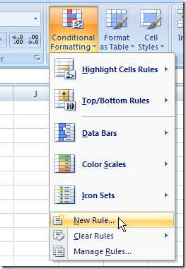
CondFormatNewRule

Create Conditional Formatting Rule

  • In the New Formatting Rule dialog box, click Use a formula to determine which cells to format
  • In the formula box, enter a COUNTIF formula, referring to the named range on the Updates sheet, and to the active cell on the All_Files sheet. Use an absolute reference to the column, $A. In this example, the formula is:
    =COUNTIF(UpdateA,$A2)
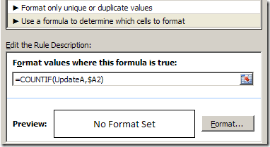
    CondFormatUpA
  • Click the Format button, and select the formatting you want for the highlighting.
  • Click OK, twice, to close the dialog boxes.

The rows for the files that have been updated are now highlighted.
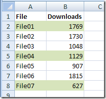
CondFormatUpGreen

You can quickly see which files are done, and concentrate on the files that still need to be updated.

Watch the Video

To see the steps in action, you can watch the following short video.

____________________

Excel Rounds Off Large Numbers-Credit Card

What danger lurks in the evil spreadsheet? Drama and tension in outer space!

No, Excel shouldn’t change your numbers, but it can happen occasionally, as this poor guy discovered.

Yes, this is silly, but it was a fun project, and the serious instructions are below the video.

Numbers in General Format

As the robot in the video mentioned, you might have problems if you try to enter a large number in Excel. For example, I’ve entered a 16-digit credit card number — 1234567890123456 — in cell A2.

Everything looks fine, until I press the Enter key.

Large number in exponential notarion number format

The cell is formatted as General, which will only display 11 numeric characters.

Since the credit card number is larger than that, it appears in exponential notation.

Significant Digits in Number Format

To make the credit card number display correctly, I could try Number format, with zero decimals.

CreditCardNumFrmt

That looks better, except that the last digit has changed from a 6 to a 0. Excel only retains 15 significant digits, so it changes our 16th digit to zero.

Large Numbers in Text Format

Since we need to see all 16 digits in the credit card number, we can format the credit card column as Text, and enter the numbers.

All 16 digits will be stored, and will display correctly.

Or, type an apostrophe before the credit card number, and it will be treated as text.

Large number in text format

More Information

On the Microsoft site, a brief article on the Number of significant digits MS Excel retains

Chip Pearson’s article on Rounding Errors In Microsoft Excel97

For smaller numbers that have been formatted as text, you can Convert Text to Numbers

____________

Create Conditional Formatting Icons in Excel

In Excel 2007, conditional formatting options include Icon Sets, such as coloured flags, stop lights, and other symbols.

These icon sets aren’t available in earlier versions of Excel, but here’s how you can create your own conditional formatting icons in Excel 2003.

TIP: You can use this technique in newer versions of Excel too, if you can’t find an existing icon set with the shapes and colours that you need

Continue reading “Create Conditional Formatting Icons in Excel”

Show More Characters in an Excel Cell

I saw this question in Twitter this week:

Anyone know a way to get an Excel cell to take over 255 characters w/o converting to pound signs ###? Wreaking havoc on something I’m trying

Cell Full of Pound Signs

First, what do you call those symbols – ###?

  • Pound signs? Hashtags? Number signs? Octothorpes?

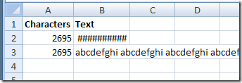
Anyway, whatever you call them, in the screenshot below, you can see an example of this 255 characters problem, in cell B2.

cells B2 and B3 contain the same long string of character

Identical Cell Content

Here’s what’s on the worksheet, shown above:

  • Cells B2 and B3 both contain an identical long string of characters.
  • In column A, a LEN formula calculates the count of characters in B2 and B3
  • The formula results in cells A2 and A3 are exactly the same:
    • There are 2695 characters in each cell

Why do the cell strings behave differently though?

  • In cell B3 the long text overflows into the next column
  • In cell B2 only the pound signs are visible.

Long Numbers

Aside from long text strings, there is another reason that causes pound signs to appear in a cell.

Those pound signs appear if a number is too long to display in a cell, and widening the column would fix that problem.

Fix the Long Text Problem

However, in this case the cells contain text, not numbers. Widening the column won’t help.

In example shown above, cell B2 is formatted as Text, and that’s what is causing the long text string problem.

There is a limit to what can show in a cell formatted as Text.

Change Cell Number Format

To fix this problem, you can change the cell’s format to General.

To change the format, follow these steps:

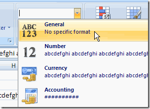
  1. Select cell B2, and on the Ribbon, click the Home tab
  2. In the Number group, click the drop-down arrow for Number format
  3. Click on General.
    • Note: If you look down the list of formats you’ll see that Accounting format and Text format show pound signs, instead of the sample text.

After you change the format, the long text string will overflow into the adjoining cell on the right.

Change to General Formal for long text strings

____________________

Excel Formatting Live Preview

One of the new features in Excel 2007 is live preview when you select a different font or theme on the Ribbon.

For example, here’s how my worksheet looks now:

Format2007_01

The default font for the cells is Calibri, and I’ve added bold in the first row.

I’m not sure if the Calibri font is the best choice, so I’d like to see how the data would look in a different font.

Select a Different Font

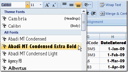
I select column H, then click the drop down arrow for Fonts on the Ribbon’s Home tab. The live preview shows the selected cells in each font as I point to it in the list.

If I find a font that I like better, I can click on it to change the font for the selected cells. None of the other cells are affected.

Excel Formatting Live Preview Font Selection

Select a Different Theme or Theme Font

In most cases, I wouldn’t just change the font in one column or a few cells. To keep the workbook from looking like a ransom note, I’d usually change the font for the entire workbook.

In Excel 2007 I can do this by choosing a new Theme or by selecting a different Theme Font.

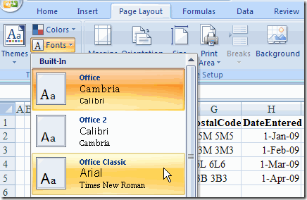
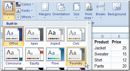
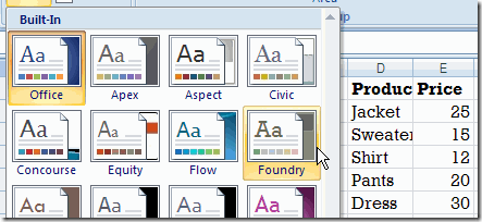
  1. On the Ribbon’s Page Layout tab, click the drop down arrow for Themes or for Fonts, then point to one of the options.
  2. The live preview affects all the cells that use the Calibri font, instead of just the selected cells.
  3. Click on one of the options and all the cells with Calibri font are changed.

Format2007_03

Formatting Converted Workbooks

Slowly, I’m converting some of my old Excel files, like the price list shown below, to Excel 2007 format.

When I use the Theme or Theme Fonts drop down list, the live preview doesn’t work. The data is still shown in Arial Narrow, which was the default font in Excel 2003.

Format2007_04

To make this worksheet fit the current theme, I’ll change the fonts to Calibri and Cambria:

  1. Click the Select all button at the top left of the worksheet, to select all the cells on this worksheet.
  2. Then, on the Ribbon’s Home tab, select the Calibri font.
  3. To format the first row as Headings, select Row 1 and apply the Cambria font.

Now, any cells that are formatted with one of the Theme fonts will show a live preview when selecting a different Theme or Theme Font.

Format2007_05

Merge Styles Tip

John Walkenbach added this formatting tip in the comments below:

“Here’s a way to quickly make an XLS workbook look like an 2007 workbook:

Open your XLS workbook, then press Ctrl+N to open a new workbook. Go back to your XLS window and activate the Merge Styles dialog (click the bottom of the scroll bar in the Styles group, then choose Merge Styles). Select the new workbook you opened, click OK, and confirm your choice.

All cells that have the “Normal” style will now be formatted in the default style for Excel 2007. In addition, the cells will respond to theme changes.”

_________________________