Cascading lists and kangaroos? Today, Ed Ferrero shares his technique for creating dependent data validation from pivot tables. Ed’s from Australia, and it looks like we’ll learn a bit about his country too, as we go through his sample file.

Dependent Data Validation
We’ve created dependent data validation drop downs before, based on named ranges, or sorted lists. Ed’s technique is perfect if you have a large data source, and it isn’t sorted in the order that you need.
In this example, there’s a list of States and Cities, with the cities in alphabetical order.

Create the Pivot Tables
Ed created two pivot tables, one with State in the row area, and one with State and City in the row area.

The State labels don’t repeat in the pivot table, so you can’t use the sorted table dependent data validation technique.
Create the Named Ranges
Instead, Ed created a couple of named ranges, and some dynamic ranges.
- The first range is State, which is the list of state names and Grand Total in the first pivot table.
- The second range is StateCity, which is the list of state names and Grand Total in the second pivot table.
Tip: If you reduce the worksheet zoom to 39%, you can see the range names.

Create the Dynamic Ranges
The first dynamic range is for the City heading in the second pivot table.
- CityHeader: =OFFSET(StateCity,-1,1,1,1)
The next two dynamic ranges, StateNo and StateCityNo, use relative references to read the value of the state from the cell to the left of the active cell. For example, if the selected State is in cell A3 on Sheet1, these formulas are used:
- StateNo: =MATCH(Sheet1!A3,State,0)
- StateCityNo: =MATCH(Sheet1!A3,StateCity,0)
Queensland is the selected State, so StateNo =3 and StateCityNo =5.
Then, the next State is found in the StateCity range.
- StateCityNext: =MATCH(INDEX(State,StateNo+1),StateCity,0)
The next State is South Australia, and it’s in row 9, so StateCityNext =9.

Create the Dependent List of Cities
Finally, the dynamic range for the list of cities is created.
- City: =OFFSET(CityHeader,StateCityNo,0,StateCityNext-StateCityNo,1)
The City range is offset from the CityHeader cell, 5 rows down, 0 columns right, 4 rows high (9-5), and 1 column wide.

Create the Drop Down List
The final step is to create the data validation drop down lists. In cell A3, a State drop down list is created, based on the State range.

In cell B3, a dependent City drop down list is created, based on the City range.

Download the Sample File
You can download Ed’s sample file to see how it works: Dependent Data Validation From Pivot Tables. It’s a zipped file, in Excel 2003 format.
About Ed Ferrero
Ed maintains an Excel techniques web site at www.edferrero.com. He is based in Australia, and has been a Microsoft Excel MVP since 2006.
____________