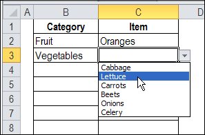
With dependent data validation, you can make one drop down list depend on the selection in another cell.
For example, select Vegetables as a category in column B, and you’ll see a drop down list of vegetables in column C.
Excel tips and tutorials

With dependent data validation, you can make one drop down list depend on the selection in another cell.
For example, select Vegetables as a category in column B, and you’ll see a drop down list of vegetables in column C.
 Data validation is one of the best features in Excel. You can use it to create drop down lists, or limit what users can enter in a cell.
Unfortunately, data validation isn’t perfect, or foolproof. Users can get around the limits, by pasting data into the cell, or by using the Clear All command in a data validation cell.
Someone sent me a question this week, asking how to trap input errors, despite these data validation failings:
In this example, an order form has two cells for dates – an Order Date, and a Delivery Date. To ensure that a date for the current year is entered, you can use formulas in the data validation, to set a minimum and a maximum date.
Start Date formula: =DATE(YEAR(TODAY()),1,1)
End Date formula: =DATE(YEAR(TODAY()),12,31)

If you’re concerned that users might paste values into the cell, or clear the data validation, you can add a formula check, to ensure that a valid date was entered.
In the order form, a date check formula is entered in column G, which can be hidden.
The formula in cell G9 is:
=OR(C9=””,YEAR(C9)=YEAR(TODAY()))
The formula is copied down to cell G10, and the result is FALSE, because the date in C10 is not in the current year.

In the Invoice total cell, the formula result is “Invalid Date”, if either of the date check cells contains FALSE. If both dates are in the current year, the total sum is shown.
Here is the formula from the Invoice Total cell:
=IF(COUNTIF(G9:G10,FALSE),”Invalid Date”,SUM(E13:E17))

Instead of a formula check, there are other ways to ensure that users enter valid data.
For example, you could use Excel VBA to check specific cells before printing, and cancel the printing if the entries aren’t valid.
Have you used other methods to ensure that users don’t ignore your data validation cells?
____________
With Excel data validation, you can create drop down lists on a worksheet. However, the font size is very small, and can’t be adjusted, and you can only see 8 items at at time.
With Excel VBA programming, you can add a ComboBox to the worksheet, to show the data validation list.
In the ComboBox, you can control the font size and the number of visible items in the list.

Although this technique works nicely in Excel 2007, and earlier versions, you might have a problem with the ComboBox size in Excel 2010.
In the screen shot below, the ComboBox is about 1/4″ wide, instead of filling the entire cell.

In other workbooks, the ComboBox is so narrow that you can’t see it at all. That’s not too helpful a feature!
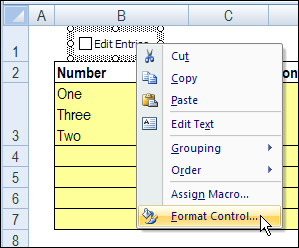
Fortunately, the problem is easy to fix in Excel 2010, if you follow these steps.
On the Developer tab, click the Design Mode command.

To select the ComboBox, type its name in the Name Box, and press Enter

On the Ribbon, under Drawing Tools, click Format, and click the Dialog Launcher for the Size group.

In the Format Shape dialog box, in the Size category, remove the check mark for Lock Aspect Ratio, and click OK
That should fix the ComboBox sizing problem!

To see the steps for changing the Size setting in Excel 2010, you can watch this short Excel video tutorial.
___________
[Latest update: July 27, 2016] With a bit of Excel VBA programming, you can change an Excel data validation drop down list, so it allows multiple selections. This post is a roundup of articles on how to set up multiple selection Excel drop down lists.
Continue reading “How to Set up Multiple Selection Excel Drop Down”
A couple of years ago, I described how you could select multiple items from an Excel drop down list. One of my clients needed that feature in a workbook last week, so I’ve made an enhancement to the VBA code. Now you can edit multiple selections in Excel after entering them.
Continue reading “Edit Multiple Selections in Excel Drop Down”
 Yes, it’s Valentine’s Day today, and if you were too busy to buy your sweetie a card yesterday, you can make one in Excel. Phew!
Your boss won’t mind if you spend a couple of hours working on this today, because it’s an Excel project! This Excel Valentine card uses a named range, data validation, a formula, and conditional formatting (to change the heart from white to pink to red).
If you won’t have time, or if your drawing skills are worse than mine, you can download the sample Excel Valentine file, at the end of this blog post.
And if you want some romantic music in the background, while you work on your Excel Valentine card, you can listen to the YouTube playlist, compiled by John Walkenbach and his blog readers.
To create the heart shape,

The formula will count how many text items have been added at the top of the worksheet, and the result is used for conditional formatting.
=COUNTA($E$1:$E$3)

With the Heart range still selected, set up the following conditional formatting:

The heart shape will be hidden, and only revealed when the Valentine message is selected.
To hide the heart:
Next, you’ll create three drop downs, for the Valentine message at the top of the worksheet.
To prepare the cells for the drop down lists:

Create the following data validation drop down lists:
Tip: To type a heart shape, press Alt and type a 3 on the number keypad (if no number keypad, try Fn+Alt+L). On a Mac, another key combination might be needed.

The Excel Valentine heart has white fill and white font, so it’s not visible.
To see the heart:

To see how the card works, you can download the Excel Valentine Card sample file.
The file is in Excel 2007 format, and zipped, and it contains no macros.
_____________
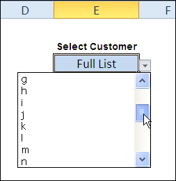
 On Monday, AlexJ showed us how to create a short or long drop down list in Excel. With his technique, users can see just the top customers, or all customers.
That technique didn’t require macros — it was driven by a formula in the data validation source.
Today, Alex shares an automated version of the short or long data validation list technique. Starting in the next section, you can read his description of how this version works.
You can download the zipped Dynamic Data Validation Sample File from the Contextures website. The file contains macros, so enable them to use the dynamic drop down list.
For an Excel utility running at our office, users are required to enter a project number using a drop down list. There are thousands of these records in the data set, selecting from hundreds of project numbers. This means that the drop-down list is long, and therefore not very useful.
To address this, we determined that the user would usually select from a short list of active projects, but would also need to select from a long list of all projects or old projects.

There are a number of techniques using dependent data validation in Excel, but these usually require two selection boxes, we wanted to do this with only a single drop down selection.
The technique presented allows the user to select from a default list of entries, or select a different list.
The two lists are named — rng.DD1 for the new projects, and rng.DD2 for the full project list. The first cell in each list is a formula, that refers to the other list.
=”>> GOTO ” & $J$3

The cell with the drop down list is named rng.DD_Select.

The result cell, $E$5, calculates which list has been selected:
=”rng.DD”&IF(rng.DD_Select=$J$3,2,1)
If the selected item matches the heading in cell J3, the result is rng.DD2, otherwise, the result is rng.DD1.

The data entry cell has data validation configured for a list, and the following formula that refers to the result cell:
=INDIRECT($E$5)

If the result in cell $E$5 is rng.DD1, the new project list is shown.

The data validation doesn’t require programming, but there is a small VBA routine triggered by the Change Event in cell B5. It tidies up the data entry cell, after a selection is made.
This routine will:

Here is the event code from the data entry sheet.
Private Sub Worksheet_Change(ByVal Target As Range)
Dim str As String
Dim strNew As String
Const strMatch As String = ">> GOTO "
If Target.Address = Me.Range("rng.DD_Select").Address Then
  str = Target.Value
  If str Like "-*" Then
    Target.ClearContents
  Else
    If str Like strMatch & "*" Then
      strNew = Right(str, Len(str) - Len(strMatch))
      Target.Value = strNew
    End If
  End If
End If
End Sub
________________
You can make data entry easier in Excel, by create a drop down list with data validation. Sometimes those lists are so long, that they become a pain to use.
Here’s a technique from AlexJ, that lets users switch between a short or full Excel drop down list of customers.
I’ve finally updated my Data Validation intro video, so it shows the steps for creating a drop down list in Excel 2010, instead of Excel 2003.
Note: These instructions apply to Excel 2007 too, in case you’re using that version.
In honour of this momentous occasion, here are links to a few of my previous Excel Data Validation articles and posts.
You probably know all the basics, but maybe you’ve missed a few of these tips and tricks.
Show or Hide User Tips In Excel – AlexJ shows how to let users turn data validation messages on or off, by choosing TRUE or FALSE from a drop down list.
Dependent Data Validation From a Sorted List – Select an item in the first drop down list, and related items are shown in the second drop down list.
Limit the Total Amount Entered in Excel – use Data Validation to limit the total amount that users enter in a group of cells.
Select Multiple Items from Excel Data Validation List – instead of selecting just one item from a data validation drop down, you can select two or more.
Plan Your Party Seating with Excel – too late for Christmas dinner, but this might help with your New Year’s festivities.
Note: Remember to vote for the Excel functions that you’d like to learn more about during the 30 Excel Functions in 30 Days challenge, starting January 2nd.
The shiny new video is below, in case you’d like to see the steps for making a drop down list in an Excel worksheet.
________________
 Can the sales staff and accounting staff ever work in peace? One group wants to see product descriptions, when entering orders. The other group thinks the descriptions clutter up the worksheet — they just want the product codes.
Try this data validation trick, and you might be nominated for next year’s Nobel Peace Prize. (Results not guaranteed.)
See the workbook details below, and there’s a video with step-by-step instructions at the end of the page.
To make it easier for users to enter data in an Excel workbook, you can create drop down lists in the cells, by using Excel data validation.

In this example the product list is in an Excel Table, and the ProductShow column is a named range — ProdList.
The ProdList range is used as the source for the drop down lists on the order entry sheet.

After the product is selected from the drop down list, the full description is automatically replaced by the product code. How does it happen?
It’s the magic of Excel VBA — event code that runs when the worksheet is changed.

The Excel VBA code uses the Match worksheet function to find the row number in the lookup list. It replaces the selected product description with the matching Product Code from that row in the lookup list.

Peace at last! Your co-workers will be happy that they don’t have to memorize the product codes, and the accounting department will be grateful that they get the data in the format they need.
To see the Excel VBA code that changes the product name to a product code, go to the Contextures website, and download the sample file: DV004: Data Validation Change.
The example used here is the Excel 2007 version, and there is also an Excel 2003 version of the sample file.
You can watch this video to see the steps for creating an Excel Table, naming a column in that table, then using that name when creating the data validation drop down list.
___________