At a client’s office last week, I was selecting a pricing option from a data validation drop down list. It had some limitations, so here are 3 types of Excel drop down lists compared.
Continue reading “3 Types of Excel Drop Down Lists Compared”
Excel tips and tutorials

At a client’s office last week, I was selecting a pricing option from a data validation drop down list. It had some limitations, so here are 3 types of Excel drop down lists compared.
Continue reading “3 Types of Excel Drop Down Lists Compared”
Garbage in, garbage out, am I right?
You depend on Excel spreadsheets to show accurate data and analysis.
Enter the wrong data and the results will be incorrect, and that could have a negative impact on your business or reputation.
Here are 3 ways to help safeguard your data entry, and I’m sure you use a few other methods in your worksheets too.
Here’s a screen shot of a data entry worksheet, where I’ve used each of those technique, to help people enter valid data.
But remember, these techniques help make your Excel files idiot resistant, not idiot proof!
You’ve met people, right? They’re very creative at finding ways around your helpful Excel data entry safeguards.

Keyboard shortcuts save you time and can prevent errors. Quickly enter the current date and time, or copy the cell above, instead of re-typing.
Instead of allowing free-form data entry, you can add drop down lists to the worksheet using the Excel data validation feature.
For example, create a list of product names, and select from that list.
This prevents typos, and only valid entries are allowed. Then, if a product is discontinued, remove it from the list, and it won’t appear in the drop down for new entries.
To create a drop down list, follow these steps:
Use a bright colour to highlight data entry cells that are empty. This makes it easy to spot the cells that have to be filled in.
To highlight an empty cell:
What techniques do you use in your Excel files, to help people enter valid data?
Do you use the 3 techniques that I listed?
___________
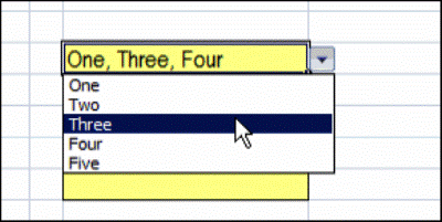
You’ve probably used an Excel data validation drop down list, where you can click the arrow, and select an item to fill the cell. With a bit of programming, you can customize a drop down list, to select multiple items.
Continue reading “Select Multiple Items from Excel Data Validation List”
You know how to create a drop down list in Excel, by using the Data Validation feature.
Sometimes you get extra fancy, and make a drop down list that depends on the selection made in another list, using dependent data validation.

Dependent data validation works well, but there’s a loophole.
In the screen shot below, I can change the category to Fruit, even though a vegetable, Cabbage, is selected as the Item in that row.
With this loophole, you could end up with some strange data on your worksheet!

Excel users are very resourceful, and can find ways around almost every safeguard that you set up.
However, you can slow them down a bit, by making the first list dependent on the second.
They’ll have to clear the Item selection before they can change the Category.
Currently, the Category cells have a data validation list that’s based on the named range, Produce.

You can change the formula in the Source box, so it only uses the Produce range if the Item cell is empty. In the screen shot below, cell B2 is active, and the Data Validation Source formula is:
=IF(C2=””,Produce,B2)

If cell C2 is empty, the Produce list will show in the drop down list.
If an Item was selected in cell C2, then the drop down list will show contents of cell B2.

It’s still not foolproof. Users could clear the Category cell, then enter any value. Or they could cut and paste from another cell.
As an extra precaution, you could add conditional formatting in column C, to turn the cells yellow if the selected Item is not in the selected Category.
With cell C2 active, the conditional formatting formula is:
=COUNTIF(INDIRECT(B2),C2)=0

The bright yellow colour will alert users if there’s an inconsistency in the selections, and make it easier for you to spot any problems.
For example, in the following screen shot, Cabbage and Rutabaga are highlighted in yellow, because the Category has been changed to Fruit.
Those items don’t appear in the range named Fruit, so the COUNTIF formula returns a zero.

This short video shows another way to block people from changing the first drop down list, if there’s a selection in the second drop down.
There are written steps, and a sample file on the Advanced Dependent Drop Down Lists page, on my Contextures site.
_________________
Roger Govier has created a sample workbook and instructions that show you how to create dynamic dependent data validation lists.
His technique lets you create multiple levels of dependent data validation, without defining a named range for each list.
Instead, Roger’s formula uses the INDEX function, with MATCH, to find a column heading, then shows the list from that column.
For example, on one sheet you can list regions, countries, areas and cities.

Then, on another sheet, select a region in column A, and see only the related countries in column B’s data validation drop down.
In column C, you’d see only the areas in the selected column, then only the applicable cities in column D.

With Roger’s technique, you’ll create four defined ranges, then use two of those ranges as the source for data validation drop down lists.
The ranges are dynamic, so you can add more items to any list, or add new lists, and the defined ranges will automatically adjust.
There are full instructions for Data Validation – Dynamic Dependent Lists, and a sample workbook that you can download.
Also, Roger Govier‘s contact information is at the bottom of that page.

____________________
In Excel, you can create a drop down Data Validation list, so it’s easy to enter valid items in a cell.
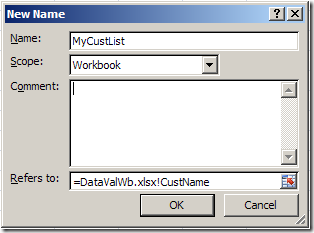
Usually, the list of valid items is stored in the same workbook, but it’s possible to set up a drop down from a list in another workbook — as long as the other workbook is open.
Continue reading “Excel Drop Down List From Different Workbook”
Today I heard from someone who was having problems with data validation, in cells that were formatted in Percent Style.
In the workbook, Enable automatic percent entry is turned on (Office button, Excel Options, Advanced, Editing options).

In the cells that are formatted as Percent Style, the percent sign automatically appears as you start typing a number.

The data validation allows Decimals between zero and 100.

All goes well if you enter a valid number in the formatted cells. However, if you enter text, or an invalid number, the Data Validation error message appears.

If you click Cancel, the cell is cleared. You can type another value in the cell, and the percent sign is automatically added.
However, if you click the Retry button, the cell isn’t cleared. The existing entry, including the percent sign, is highlighted.
When you type a new number, it replaces the existing entry, and Excel doesn’t automatically add a percent sign.
The result is a percentage much higher than what you intended. Here, it’s 5500% instead of 55%

If you use the Retry button, remember to type the percent sign yourself.
Or, click Cancel, to start a new entry.
As a reminder, you could add those instructions to your Data Validation error message.
Or, turn off the Enable automatic percent entry option, and always add a percent sign if typing a whole number in these cells.
There’s more information on the Enable automatic percent entry option in the Microsoft Knowledgebase.
__________________
You can use Excel’s Data Validation to limit the total amount that users enter in a group of cells.
For example, if budget is $3500, you can prevent entries that will go over that total amount.

Here’s what is on the Budget data entry sheet:
On the Budget Data Entry Sheet, data validation is applied to cells C3:C7, because this is where the data entry occurs.


After setting up the data validation, you can test it, to make sure that it works as expected.

_______________________
To help users enter data in a spreadsheet, you can create drop down lists with Excel’s Data Validation feature. For example, in an order form, you could provide drop down lists of customers, products, colours, sizes and shipping methods.
Usually, each of these lists would need a different Source in the Data Validation dialog box.

Instead of using a different source for each data validation list, AlexJ has devised a simple way to use the same source for all the lists. This makes it much easier to create and maintain a set of drop down lists.
In AlexJ’s sample file, he’s recording farm information, with drop down lists for Fruit, Vegetable, Farm Equipment and Farmer. He’s typed these lists in the workbook, and named them: DD.Fruit, DD.Veg, DD.Equip and noDD.
The noDD list is just a blank cell, and it can be used when you want users to be able to type freeform in a column.

In row 2, above the table where users will select from the drop down lists, AlexJ has typed the name of the source range for the column below.

Then, AlexJ selected all the blue cells, where drop down lists will be created. In the Data Validation dialog box, he selected Allow: List. As the Source, he entered: =INDIRECT(C$2)
The column reference (C) is relative, and the row reference ($2) is absolute.

To download AlexJ’s sample file click here: Universal Data Validation Drop Downs (zipped 25 KB)
I frequently use the INDIRECT function to create dependent data validation lists. However, I hadn’t seen this idea used before, to create different drop down lists from the same source formula.
To me, it seems like a great way to create several adjacent lists, and makes it easy to maintain them.
AlexJ would appreciate your feedback. What do you think? Would you use this technique? Anything you’d add or change?
_________________________
When you set up a worksheet for other people to use, data validation messages can help them get started. The messages appear, like little ToolTips, when a user clicks on a cell.
After using the Excel workbook for a while, users might not need those messages anymore, and the pop-up messages become annoying, rather than helpful.
AlexJ, who recently shared his technique for hiding rows with Excel outlining, has created another useful sample.
In this file, he lets users turn those data validation messages on or off, by choosing TRUE or FALSE from a drop down list.

When TRUE is selected, the label cells, such as Name, are green. Click on a label cell and a data validation input message appears, with instructions for that field.

Select FALSE and the label cells turn white, and no data validation input message appears when you click on a label cell.

The TRUE/FALSE drop down list is in a cell named ShowUserMsg, and the list is created with data validation.

The labels cells also have data validation, which is set to allow Any value.

For each label, an Input Message is entered in the Data Validation dialog box.

The label cells and ShowUserMsg cell are coloured with Conditional Formatting.

When you select an option from the TRUE/FALSE list, a Worksheet_Change event runs, and turns the messages on or off.
To see the code in Alex’s sample file, right-click the Show User Messages sheet tab, and click on View Code.

You can download the Show or Hide Messages file from AlexJ’s Sample Spreadsheets page on the Contextures website.
In the Data Validation section, look for DV0001 – Show or Hide User Tips
___________________