What will you do better in Excel next year? Do you have any Excel bad habits that you’ll break? Are there any Excel skill areas that you’ll improve?
Excel Resolutions
Based on the questions that I see in the Excel newsgroups and forums, lots of people could resolve to do one or more of these things:
Save your Excel files every few minutes as you work on them. Jan Karel Pieterse has a terrific (and free) Excel add-in – AutoSafe – that will automate the saves for you, and it’s way better than Excel’s built in autosave feature.
Make backup copies of every important Excel file, and update those backups regularly. Yes, something will go wrong eventually, and those backups are lifesavers.
Add an instruction sheet to your key Excel files and complex worksheets. Then, if you’re away for a holiday, your co-workers won’t have to call you with frantic questions, or mess things up on their own. Maybe that’s what happened to the banking industry.
My Excel Resolutions
Here are my Excel goals for 2010:
Spend a couple of hours each week working with the Excel 2010 beta, and PowerPivot for Excel add-in, so I’m ready to roll when the final version is released.
Make better notes when I write and edit code. Sometimes it’s clear what the code is doing, but I can’t remember why I decided to do things a specific way. A few notes could save time and frustration later.
Update my Pivot Table add-in so all the features work in Excel 2007. Jon Peltier is planning a series on creating Excel add-ins, so that could give me some ideas for improving my add-in.
Your Excel Goals for 2010
What about you? Do you have an Excel goals for 2010 that you’d like to share?
Making your Excel resolutions public might help you stick to them!
____________
A bit of Excel programming can help us save some time and paper. Our goal is to stop people from printing an order form if they forgot to enter a customer name.
Final Macro Changes
Last week, you created a macro to show a message if the customer name was missing in an order form.
Today, you’ll make a final change to the macro, so it will run automatically when someone tries to print the order form.
Sample File: You can download the Excel order form with last week’s message macro. Enable macros when the file opens.
Create the Event Code
To create Excel code that runs automatically, you can use Event procedures. Those are macros that run when something specific happens in Excel, such as changing a cell on a worksheet, or printing a worksheet.
To open the Visual Basic Explorer (VBE), right-click on the Order Form sheet tab, then click View Code.
Create the Event Code
In the VBE, find the order form workbook in the list of projects, and under Microsoft Excel Objects, double-click ThisWorkbook.
At the top left of the Code Window, select Workbook from the drop down list.
An event procedure for Workbook_open is automatically created, but that’s not the one we need, so just ignore it. At the top right of the Code Window, select BeforePrint from the drop down list.
The cursor should be flashing between the Sub and End Sub lines for the Workbook_BeforePrint macro. We want to check the order form before someone prints it, so type the following 2 lines of code, to check the name of the active sheet:
Next, copy the code from the CustomerMessage macro, on the Module1, and paste it between the If and End If lines.
Now, when someone tries to print or print preview, Excel will check the sheet name.
If OrderForm is the active sheet, it will check for a customer name in cell B5.
If the customer name is missing, our warning message will appear.
Test the Event Code
To see if the BeforePrint code is working correctly, you can test the code by using Print Preview.
On the Order Form worksheet, delete the Customer Name in cell B5.
Click the Office Button, point to Print, then click Print Preview.
The good new is that the warning message appears, because the Customer Name cell is empty. The bad news is that the Print Preview opens, even though the customer name is missing.
Fine-Tune the Event Code
You can see “(Cancel as Boolean)” at the end of the first line in the Workbook_BeforePrint macro. Some Excel events have a Cancel option, which allows you to cancel the event, if necessary.
We’ll add one more line of code, to cancel the printing if the customer name is missing.
In the Workbook_BeforePrint code, add a blank line, after the MsgBox line.
In the blank line, type: Cancel=true
Then, save the workbook, and try the print preview again.
Now the warning message should appear if the customer name is missing, and the print or print preview should be cancelled.
If the customer name is filled in, then no message will appear, and the order form will print, or show up in the print preview window.
_________________
How long is your attention span? It’s a short work week, so let’s start it off with a couple of quick Excel tips. And when I say “Quick,” I mean, “Don’t blink, or you’ll miss them.”
I recorded a few quick Excel tips, and posted them in the Excel Quick Tips playlist on my Contextures YouTube channel.
If you can’t sit still through a lengthy 2 minute video, this might be the solution!
Select a Random Name
The first video shows you how to select a random name from a list. Enter the RAND function in the column adjacent to the list of name.
Then, sort the column with the RAND function, and the name at the top is the winner.
This is the same technique that I used to select winners in my Excel Summer Giveaway and Excel Fall Giveaway contests.
Keeping Excel users on the right path is a big job, but somebody’s got to do it!
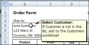
Last week we created an Excel message box in an order form, to remind users to select a customer name.
However, we don’t want the message to appear in every order form – it should only show if the customer name cell is empty. We’ll modify the code so it checks for a customer name.
Sample File: You can download the Excel order form with last week’s message macro. Enable macros when the file opens.
Clear the Customer Name Cell
To see how to refer to the customer name cell, we’ll record a test macro.
Select any sheet in the workbook, other than the OrderForm sheet.
Start the Macro Recorder
Name the macro NameTest, and store it in This Workbook
Click on the OrderForm sheet tab, to activate that sheet
Select cell B5, where the customer name is entered
Stop the Macro Recorder
Clear the Customer Name Cell
To see the recorded macro:
On the Ribbon, click the View tab
Click Macros, then click View Macros
In the list of macros, click NameTest, then click Edit.
Here’s the recorded code, with the comment lines and blank lines removed. It shows you how to refer to a sheet and cell in Excel VBA code.
We’ll remove the Select in each line, and combine the two lines into one. At the end of the line, add: .Value = “”
The revised line of code will set the value of the customer name cell to an empty string.
Run the NameTest macro, and it should clear the customer name cell.
Check For a Customer Name
We’ll add the new code to the old code, that shows the message. To check for a customer name, we’ll create an IF…THEN section in the macro, similar to what you’d do in an IF formula on the worksheet.
In English, the instructions would be: IF the customer name cell is empty, THEN show the message. In the Excel VBA code, we’ll use these three lines:
Now, when you run the CustomerMessage macro, you should see the message box only if the customer name cell is empty.
The Next Step
Next week, we’ll add code to make the macro run automatically, when someone tries to print the order form.
_________________
Previous Excel VBA articles:
Should you spend extravagantly this Christmas, or go cheap, or spend somewhere in the middle?
You can use Excel Scenarios to store several versions of a budget, and compare the results. Let’s set up a worksheet where we can compare three scenarios for holiday spending.
Set Up the Worksheet
The first step is to set up the worksheet. Some of the cells will be the same in each Excel scenario, and other cells will change.
Note: There’s a limit of 32 changing cells in an Excel Scenario.
On a worksheet named Budget, add headings, spending categories, and amounts, as shown in the screen shot below.
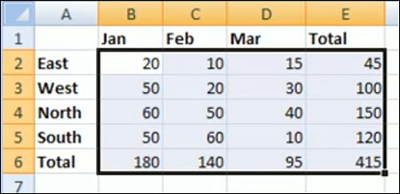
Add a Total label, and a sum of the spending amounts.
Excel Scenario for Extravagant holiday budget
Create the First Scenario
The first scenario is for Extravagant spending, which will contain the highest amounts.
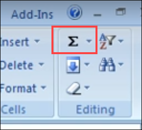
On the Ribbon, click the Data tab.
Click What-If Analysis, then click Scenario Manager. (In earlier versions, click Tools>Scenarios)
In the Scenario Manager, click Add
Type name for the Scenario. For this example, use High.
Clear the Changing cells box
With the cursor in the Changing cells box, click cell B4 on the worksheet. That’s one of the cells that will change in each scenario.
Hold the Ctrl key, and select cells C6:C11. Do not include any of the category labels, or the total cells.
(optional) Enter a comment that describes the scenario.
Click OK to close the Edit Scenario box.
Add the Scenario Values
The Scenario Values dialog box opens, with a box for each changing cell. It automatically displays the current value in each changing cell. You could modify one or more of the existing values, or leave them as is.
We’ll make the Gifts – Family amount a bit higher, and leave the other values untouched.
For item 5, change the value from 500 to 600.
Click OK to return to the Scenario Manager. Notice that the value on the worksheet didn’t change – it still shows 500 as the amount for Gifts – Family.
Add Excel Scenario values
Create Another Scenario
You can add more scenarios by changing the worksheet values, and following the steps that you used to build the first scenario.
Or, you can add an Excel scenario directly into the Scenario Manager.
In the Scenario Manager, click Add
Type name for the next scenario. For the second scenario, use Mid.
Leave the existing cells in Changing cells box
(optional) Enter a comment that describes the second scenario.
Click OK to close the Add Scenario box.
In the Scenario Values dialog box, enter the worksheet heading and values for the second scenario.
Click OK to return to the Scenario Manager.
Create the third scenario – Low – and enter the lowest amounts for that scenario.
Click Close, to return to the worksheet.
Show a Scenario
Once you have created the Excel Scenarios, you can show them.
On the worksheet, the original values for Extravagant scenario are showing.
To change to a different scenario, follow these steps:
On the Ribbon, click the Data tab.
Click What-If Analysis, then click Scenario Manager. (In earlier versions, click Tools>Scenarios)
In the list of Scenarios, click on a Scenario name
Click the Show button, then click Close.
Show a Scenario
Show the Excel Scenario Summary
After you create the Excel Scenarios, you can view them in an Excel Scenario Summary. This lets you see the values and totals side-by-side, for an overall comparison.
Note: The Excel Scenario Summary does NOT update automatically if you change the scenario values. You can delete the old summary and create a new one.
To create a Scenario Summary:
On the Ribbon, click the Data tab.
Click What-If Analysis, then click Scenario Manager. (In earlier versions, click Tools>Scenarios)
In the Scenario Manager, click Summary
In the Scenario Summary dialog box, for Report type, select Scenario Summary
Click in the Result cells box, and on the worksheet, click the Total calculation cell (C12).
Click OK, to close the dialog box.
A Scenario Summary sheet is added to the workbook.
To show or hide the details, click the + / – buttons at the left side and top of the worksheet
Improve the Scenario Summary
In the Scenario Summary shown above, the changing cells are shown as addresses.
If you name the value cells, the Scenario Summary will show those names, instead of the cell addresses.
You could probably change the colour scheme too, unless you’re a big fan of grey and purple!
P.S. There’s more information on Excel Scenario Summary settings, and programming examples, on my Contextures website.
___________________
In Excel 2003 and earlier versions, you can use an Advanced Filter to remove duplicates. In Excel 2007, there’s a new command on the Ribbon to make it easier to remove duplicates from a list.
Be careful with the Excel 2007 Remove Duplicates feature though – it really removes the duplicates. If you use an Advanced Filter instead, you have the option of hiding duplicates, or creating a unique list in a new location.
How It Works
Update: Jason Morin asked a few questions about the Remove Duplicates feature, and how it works, so I’ll answer the questions here. (Thanks Jason!)
1) Does the new Duplicates capability discern between text strings and numerical values that look the same on the screen?
No, it treats the text strings and numbers the same. If the list has a 10 and a ’10, they’ll be treated as duplicates. There isn’t a settings option that I can see, where you can adjust this. In the Advanced Filter feature, those would be seen as 2 unique items.
2) What about non-visible characters in the cell? Does it consider “Pen” and “Pen ” the same? As a user I would view this as a duplicate, but Excel may not.
No, those won’t be treated as duplicates, because the space character in the second entry makes it different. Advanced Filter would do the same.
3) How does it decide WHICH duplicate to remove in the data set?
The first instance of each item is left, and all subsequent entries are deleted.
4) I assume if I’m working with record set (>1 column), I need to concatenate data from columns to create a unique identifier for each record, then run the Duplicates on the new column I created.
You can use the check marks in the Remove Duplicates dialog box, and select all the columns you want to include. Only if all the included columns are duplicated, will an item be removed. Advanced Filter works the same way, but without the check marks.
Remove Duplicates
In this example, the list in cells A1:A10 contains a few duplicates.
Follow these steps to remove the duplicates.
Select any cell in the list, or select the entire list
On the Ribbon’s Data tab, click Remove Duplicates.
In the Remove Duplicates dialog box, select the column(s) that you want to remove duplicates from
Check the box for My Data Has Headers, if applicable, then click OK.
Remove Duplicates dialog box
A confirmation message will appear, showing the number of duplicates removed, and the number of unique items remaining. Click OK to close the message.
Watch the Remove Duplicates Video
Here’s a very short video that shows the steps to remove duplicates in Excel 2007.
Unfortunately, no one has found a way to zap users with a mild shock from the keyboard, so we have to rely on messages to help people do the right things in Excel.
Let it snow! One of the advantages of working from home in Canada, is that you don’t have to go out in rush hour, on snowy days. I can sit in my office, basking in the glow of the computer monitor, mesmerized by the flickering of the modem lights.
But eventually I’ll have to go out to do some shovelling, in the sub-zero temperatures. Later, while thawing out, I’ll create an Excel file, to track the miserable temperature and snowfall accumulation.
A Matter of Degree
We record our temperatures in Celsius, while our neighbours in the USA use a Fahrenheit scale. So, while I’m shivering on a -10°C day, it seems much warmer across the lake, where it’s a balmy 8°F.
I’m sure there are good reasons why the USA didn’t switch to the metric system when Canada did, but for now, we can use Excel to convert the temperatures.
Use Arithmetic
Maybe the temperature in the USA really isn’t as warm as it seems.
To convert the temperature from Fahrenheit to Celsius , you can use this formula:
°C = (°F – 32) x 5/9
If the Fahrenheit temperature is in cell B2, put this formula in cell C2:
=(B2 – 32) * 5/9
When I convert that balmy 8°F, it makes me feel better – it’s actually colder there, at -13°C.
Let Excel Convert It
That formula isn’t too difficult, but it might be hard to remember if your brain is affected by the cold weather. An easier way to convert the temperature is to use Excel’s CONVERT function.
Note: If you’re using Excel 2003, or an earlier version, you’ll need to install the Analysis ToolPak to use the CONVERT function.
Excel CONVERT Function
With the CONVERT function, you refer to the cell that contains the amount that you want to convert. Then you enter the original unit of measurement, and then the new unit of measurement.
We want to convert the value in cell B2, from Celsius (“C”) to Fahrenheit (“F”).
=CONVERT(B2,”C”,”F”)
Later, I can use CONVERT to see how many inches of snow we got, when the weather channel reports the snowfall in centimetres.
Excel Help for CONVERT Units
If you aren’t sure what code to use for each unit of measurement, you can check the list in Excel’s help for the CONVERT function.
Excel Help for CONVERT Units
Now I have to go and figure out how many glasses of wine are in that 750 ml bottle. I think the answer might be – not enough!

 What will you do better in Excel next year? Do you have any Excel bad habits that you’ll break? Are there any Excel skill areas that you’ll improve?
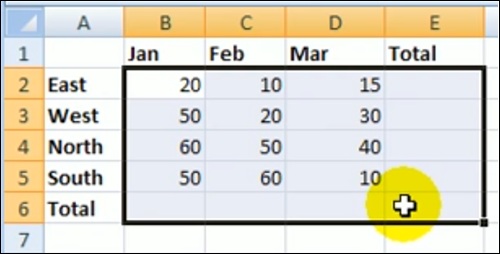


 We record our temperatures in Celsius, while our neighbours in the USA use a Fahrenheit scale. So, while I’m shivering on a -10°C day, it seems much warmer across the lake, where it’s a balmy 8°F.
