Automatically Change Excel Filter Heading

techrepublic There was a question about Excel Advanced Filter criteria on the Tech Republic blog recently, and I posted an answer.

A couple of weeks later, a Tech Republic mug and flag were delivered to my door, as a reward for answering.

It’s a Fragile Major Award

The real joy is in solving a problem, but it’s fun to get a major award, even if it’s not a fancy leg lamp that I can put in the front window.

Keep reading, to see what problem the blogger was having with Excel Advanced Filters, and download a workbook with my suggested solution.

Set Up an Advanced Filter

To use an Excel Advanced Filter, you create a criteria range, with headings that match the ones used in the original table.

Then, under one or more of the headings, you enter the filter criteria.

For example, in the screenshot below, the criteria would extract all the records where the quantity ordered is 20 and the product is juice.

With an Advanced Filter, you can even extract the data to a different location, all in one step.

Advanced Filter Dialog Box

Identical Headings

In most cases, when you set up an Advanced Filter criteria range, each heading must be identical to a heading in the source data table.

An easy way to make them identical is to link from the criteria headings to the table headings.

In the screenshot below, cell F1 has a formula with a link to cell B1.

  • =B1
cell F1 has a formula with a link to cell B1

Different Headings

However, there’s one situation in which the criteria range headings must NOT match the table headings — if you use a formula in the criteria row.

In the example below, we’d like to extract the records where the number ordered is different than the number shipped.

In the criteria range, there’s a formula in cell G2, to compare the quantity ordered and quantity shipped.

  • =C2<>D2

Remove Criteria Heading

For this filter to work, the heading in cell G1 has to be removed, or changed to something different than any of the table headings.

AdvFilterHead04

Add a Space Character

Another option would be to leave the link to the table heading, and add a space character or underscore. That extra character makes the headings different

  • =C1 & ” “

AdvFilterHead05

Create Adjustable Criteria Headings

This was the problem that the Tech Republic blogger encountered — remembering to manually change the heading, or remove it, when using a formula in the criteria range.

The question posed included this restriction:

Remember, you don’t want to force users to remember that in this particular case… they have to do something special like delete header text! Working with the list and criteria ranges, already in place, how would you get the desired results?

Heading With IF Formula

To make the heading adjust automatically, you can use an IF formula to test what’s in the cell below.

=C1 & IF(ISLOGICAL(G2), “_” , “” )

If cell G2 contains TRUE or FALSE, then it has a criteria formula, and an underscore is added to the heading.

AdvFilterHead06

Download the Advanced Filter Workbook

To see the data and the criteria range heading formulas, you can download the Advanced Filter Criteria Headings sample file. It’s in Excel 2003 format, and zipped.

The file contains a macro, that lets you run the advanced filter by clicking the Filter button on the worksheet. Enable macros if you want to use that feature.

AdvFilterHead07

Watch the Advanced Filter Criteria Video

To see the steps for applying an Advanced Filter, with regular criteria or a formula in the criteria range, please watch this short Excel video tutorial.

___________

Add Filter Markers in Excel Pivot Table

If you’re using Excel 2007 or Excel 2010, you can quickly see which fields in a pivot table have filters applied.

For example, in the screenshot below, the ItemSold field has been filtered.

The arrow drop down has changed to a filter symbol, with a tiny arrow.

pivotfiltermarkers00

Earlier Excel Versions

In Excel 2003 though, there’s no indicator that a field has been filtered. Here’s the same filtered pivot table in Excel 2003, and the drop down arrows look the same in both of the fields.

There’s no marker to show if either field has been filtered. You’d have to click each arrow, to see if any of the check marks have been removed from the pivot items. Who has time for that?

pivotfiltermarkers02

Create Your Own Filter Markers

Several of my clients are still using Excel 2003, and maybe you use it too. If so, you’ll appreciate this sample Excel file from AlexJ, which adds a bright blue marker above each filtered field.

That makes it easy to keep track of what’s been changed in the pivot table, and prevents you from overlooking the filters.

  • Tip: You could even use these markers in newer versions of Excel. The bright blue arrows are easier to see than the tiny filter icons!

pivotfiltermarkers03

User Defined Function

To create the markers, Alex wrote a user defined function, named pvtFilterID.

In the screenshot below, you can see the pvtFilterID formula in cell D5, which refers to the ItemSold field heading in cell D7.

=pvtFilterID(D$7)

The formula is used in cells B5:D5, above the row fields, and that range could be adjusted if your pivot table has a different number of row fields.

Filter Markers for Excel Pivot Table

The Blue Arrow Marker

Cell D1 is named Symbol.Filter, and it contains the blue arrow symbol that’s used as a marker.

If you changed the symbol there, the new symbol would be used as the filter marker.

In cell G5 there’s another formula, that shows a message if any of the pivot table fields are filtered.

  • =IF(COUNTIF($B$5:$D$5,Symbol.Filter)>0, “Pivot Filter On” & Symbol.Filter,””)

This formula checks the cells above the pivot table, and shows the message if any of those cells contain the marker symbol.

Works With Slicers Too

Even though Alex wrote this code for Excel 2003 pivot tables, it works in Excel 2007 and Excel 2010 too.

In the screenshot below, you can see and Excel 2010 pivot table with slicers, and the filter markers highlight the row fields where filters have been applied.

The filter symbol is on the field drop downs too, and the bright blue markers are extra insurance that users notice which fields are filtered.

pivotfiltermarkers04

The Filter Marker Function Code

Here’s Alex’s code for the pvtFilterID function.

Function pvtFilterID(rng As Range) As String  'rng As Range)
On Error GoTo XIT ' -not in pivot
If Not rng.Parent Is ActiveSheet Then GoTo XIT
If rng.Cells.Count > 1 Then
    MsgBox "Error: pvtFilterID range selection"
    GoTo XIT
End If
If rng.PivotField.HiddenItems.Count > 0 Then
    pvtFilterID = [Symbol.Filter]
End If
XIT:
End Function

Clear the Pivot Table Filters

Another nice feature that was added to Excel 2007 pivot tables is the Clear All Filters command. Alex’s workbook contains a button that runs code to remove all the filters from a pivot table.

Here’s the code for the ClearPivotFilters procedure.

Sub ClearPivotFilters(ws As Worksheet)
    Dim pvt As PivotTable
    Dim pf As PivotField
    Dim pi As PivotItem
    Dim lSort As Long
On Error Resume Next
Set pvt = ws.PivotTables("PivotTable1")
For Each pf In pvt.VisibleFields
    If pf.HiddenItems.Count > 0 Then
      lSort = pf.AutoSortOrder
      pf.AutoSort xlManual, pf.SourceName
      For Each pi In pf.PivotItems
        pi.Visible = True
      Next pi
    End If
    pf.AutoSort lSort, pf.SourceName
Next pf
Set pi = Nothing
Set pf = Nothing
Set pvt = Nothing
End Sub

The button code passes the worksheet name to the procedure.

Private Sub cmdClearPvtFilters_Click()
    Call ClearPivotFilters(Me)
End Sub

Download the Sample File

To test the pivot table filter markers, and see the VBA code, you can download Alex’s sample file from the Contextures website.

On the AlexJ Sample Files page, go to the Pivot Tables section, and look for: PT0000 – Pivot Table Filter Markers
___________

Show Us Your Spreadsheets

showspread03a Another humdrum day in the world of spreadsheets? Hardly!

Thanks to John Walkenbach (Mr. Spreadsheet) and Mike Alexander (DataPig), things are getting exciting.

They’ve just announced a Show Us Your Spreadsheets contest, with Excel books and gift cards going to the winners. The contest is open to residents of the USA, UK, and Canada (except Quebec).

How to Enter

To enter, send in a photo of yourself with one of John’s or Mike’s books, or with a fabulous Excel workbook that you created.

As an example of creative book holding, here’s John hiding behind a notebook, imitating the poses of his buddies Bill and Steve.

showspread02

Read the Rules

Be sure to read and follow the official rules, and submit your photos (up to 3) by December 3rd.

You probably have some Excel books by John and/or Mike, but if not, head to Amazon or your local bookstore, and pick one up (or a bunch!)

books_only

Picking the Winners

The best photos will be selected by John and Mike, and prizes awarded based on their decision. These multi-talented gentlemen have previous experience in judging creative events, as you can see in the photo below.

Dick is constructing an amazing tower, and you can see John (second from left) and Mike (right), judging the event. This shows that they have a keen eye for design, and are calm in the face of danger.

They seem to like beer and hockey pucks too, so that bodes well for the Canadian entries!

showspread01
____________

Get Date Year Month Day With Excel Functions

Sometimes, working with an Excel data import can be a rocky horror (text) show. This month, I’ve been working with a client who is pulling together data from several accounting systems.

The project is extra exciting because each system stores the data in a different format, and we have to assemble it into a common file.

I’m sure you’ve had to deal with a similar challenge, and used your mad scientist Excel skills to clean up the mess.

Imported Data – Date Formats

In one of the import files that my client uses, the date is stored in a YYYYMMDD format.

From that number, we have to calculate the transaction date, so Excel can understand it.

You can use a few Excel functions to extract the year, month and day, and turn that time warp into a valid date.

To quote the “Time Warp” song lyrics:

  1. It’s just a jump to the LEFT
  2. And then a step to the RIGHT
  3. Put your hands on your MID (hips)

Get Year with LEFT Function

In the screen shot below, the imported date is in column A. The year is at the left, in the first four characters.

Use the Excel LEFT function to pull those 4 digits into column C, to show the year.

  • =LEFT(A2,4)
Get Year with LEFT Function

Get Day with RIGHT Function

The transaction day is shown in the two characters at the right of the date in column A.

Use the Excel RIGHT function to pull those two digits into column E, to show the day.

  • =RIGHT(A2,2)
Get Day with RIGHT Function

Get Month with MID Function

The final step is to use the Excel MID function to pull a specific number of characters from the middle of the string in cell A2.

The month number starts at the 5th character, and is 2 characters long.

  • =MID(A2,5,2)
Get Month with MID Function

More Excel Text Functions

To see a few more Excel text functions, and a sample workbook, you can visit the Split Address With Formulas page on my Contextures website

Also, see the see the Date Format Troubleshooting Tips page, for date troubleshooting tips.

Watch the LEFT, RIGHT, MID Video

To see the steps for using the LEFT, RIGHT and MID functions in Excel, to get a valid data from a date string, you can watch this short Excel video tutorial.

____________

Celebrating VLOOKUP Week

image Over at Chandoo’s Excel blog, he’s celebrating VLOOKUP week, with helpful posts like VLOOKUP Formulas Go Wild. Who knew an Excel formula could go wild?

I’ve seen many workbooks where things have run amok, but fortunately, Chandoo’s examples are much better behaved.

Excel VLOOKUP Videos

You don’t need any special equipment or fancy telescopes to do a lookup in Excel — you just need a simple formula.

In my videos below, see how to use the VLOOKUP function, and overcome its few shortcomings with other functions, like INDEX and MATCH.

Watch the VLOOKUP Videos

I’m a big fan of VLOOKUP too, and have made several Excel VLOOKUP videos that show you how to use the function in different scenarios.

First, here’s a video that shows a basic VLOOKUP formula to get the correct price from a product price lookup table.

___

Excel MATCH Function with VLOOKUP

Next, here’s a video that shows you how to use the Excel MATCH function within a VLOOKUP formula, to make it more flexible.

Approximate Match in VLOOKUP

The next video show you how to use VLOOKUP to change a student’s numeric score into a letter grade, by using the Approximate Match option.

More VLOOKUP Tips and Videos

You can head over to my Contextures website, and see more VLOOKUP function examples and videos.

That page also has tips for troubleshooting VLOOKUP problems, like the formulas shown in the screen shot below.

After the list was sorted, the VLOOKUP formulas ended up in the wrong order, and show the wrong product prices!

VLOOKUP returns incorrect result after sorting

Celebrate VLOOKUP Weekend

With all this information on VLOOKUP to read and watch, you won’t have to worry about planning any other weekend activities.

Chandoo’s VLOOKUP Week might end today, but you can continue celebrating, by creating your own VLOOKUP Weekend. Have fun!
____________

Excel Drop Down List With Product and Code

image 
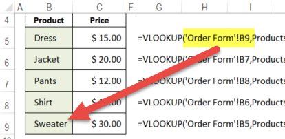
Can the sales staff and accounting staff ever work in peace? One group wants to see product descriptions, when entering orders. The other group thinks the descriptions clutter up the worksheet — they just want the product codes.

Try this data validation trick, and you might be nominated for next year’s Nobel Peace Prize. (Results not guaranteed.)

See the workbook details below, and there’s a video with step-by-step instructions at the end of the page.

Create Drop Down Lists

To make it easier for users to enter data in an Excel workbook, you can create drop down lists in the cells, by using Excel data validation.

Excel Drop Down List With Product and Code

Product Lookup Table

In this example the product list is in an Excel Table, and the ProductShow column is a named range — ProdList.

The ProdList range is used as the source for the drop down lists on the order entry sheet.

DataValProdCode01

Add Excel VBA Magic

After the product is selected from the drop down list, the full description is automatically replaced by the product code. How does it happen?

It’s the magic of Excel VBA — event code that runs when the worksheet is changed.

DataValProdCode03

Drop Down List VBA Code

The Excel VBA code uses the Match worksheet function to find the row number in the lookup list. It replaces the selected product description with the matching Product Code from that row in the lookup list.

DataValProdCode04

Peace at last! Your co-workers will be happy that they don’t have to memorize the product codes, and the accounting department will be grateful that they get the data in the format they need.

Download the Sample File

To see the Excel VBA code that changes the product name to a product code, go to the Contextures website, and download the sample file: DV004: Data Validation Change.

The example used here is the Excel 2007 version, and there is also an Excel 2003 version of the sample file.

Watch the Data Validation Video

You can watch this video to see the steps for creating an Excel Table, naming a column in that table, then using that name when creating the data validation drop down list.

___________

Excel VBA Click Shape to Sort Column

People are lazy! Shocking, I know, but who wants to click twice in Excel, if you can do the same thing by only clicking once?

SortClick00

Click to Sort Column

Peterson, champion of weary Excel users, created this sample Excel VBA sort code, that adds invisible rectangles at the top of each column in a table.

A macro is automatically assigned to each rectangle, and it sorts the table by that column, when you click it.

Benefits of Sort Macros

Here are two benefits of using Dave’s code:

  1. Reduced wear and tear on clicking fingers
  2. Less risk of table scrambling, because it ensures the entire table is selected before sorting
Click Invisible Shapes to Sort Columns

Edit the Setup Macro

There are two macros in Dave’s sample file.

  • SetupOneTime – run this once, to add the hidden rectangles
  • SortTable – sorts table by selected column, when heading is clicked

Before you run the SetupOneTime macro, you should edit both macros, to adjust them for your workbook

  1. On the Excel Ribbon, click the Developer tab, then click Macros
  2. Click SetupOneTime, and click Edit

SortClick02

The Setup Macro Code

In the SetupOneTime macro, change the iCol variable to match the number of columns in your table. If your table doesn’t start in cell A1, change that reference.

SortClick03

Edit the SortTable Macro

Next, change the variables in the SortTable macro, to suit your table settings. You can adjust:

  • TopRow (row where headings are located)
  • iCol (number of columns in the table)
  • strCol (column to check for last row)

SortClick04

If you want to see the rectangle outlines, change the Line.Visible setting to True.

SortClick06

Run the SetupOneTime Macro

After you’ve edited the macros, you can run the setup macro:

  1. Select the sheet where your table is located.
  2. On the Excel Ribbon, click the Developer tab, then click Macros
  3. Click SetupOneTime, and click Run

SortClick07

Now, click a heading in the table, to sort by that column.

Excel 2007 Shapes Problem

When I was getting this blog post ready, I discovered that Dave’s original code needed a tweak before it would work correctly in Excel 2007 and Excel 2010.

In the original code, written for Excel 2003, there was one line of code that made the rectangular shape invisible:

.Fill.Visible = False

In the newer versions of Excel, only the borders of the invisible shapes were clickable, so I had to change the code to these two lines:

.Fill.Solid
.Fill.Transparency = 1#

The revised code worked for me in Excel 2003, 2007 and 2010, creating transparent shapes that were clickable.

SortClick05

Download the Sample Workbook

To see the full code for the SetupOneTime and SortTable macros, and download the sample workbook, visit the Sort Data With Excel Macros page on the Contextures website.

And for more Excel advanced sorting tips, go to the Excel Add-in Advanced Sorting page on my Contextures site.

Watch the Click Headings to Sort Columns Video

To see the steps for editing the code, adding the rectangles, and clicking the hidden shapes, you can watch this short Excel tutorial video.

_________________