How to Find MIN IF or MAX IF in Excel

When you were first learning how to use Excel, you quickly discovered the basic Excel functions, like SUM, COUNT, MIN, MAX, and AVERAGE. Now you’re ready for advanced calculations, like how to find MIN IF or MAX IF in Excel.

Beyond the Basics with MIN IF

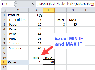
In this example, we want to see the MIN and MAX for a specific product. There is a SUMIF function and a COUNTIF function, but no MINIF or MAXIF.

• [Update]: In Excel 2019, and Excel for Office 365, you can use the new MINIFS and MAXIFS functions. There is more information on the MIN and MAX page on my Contextures site.

So, we’ll have to create our own MINIF formula, using MIN and IF. I’ve selected a product in cell C11, and the formula will be built in cell D11.

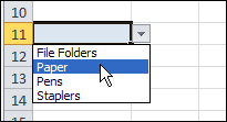
To make it easy to select a product, I created a drop down list of product names, by using data validation.

NOTE: You can also calculate MIN IF and MAX IF with Multiple Criteria

MIN IF Formula

The formula starts with the MIN and IF functions, and their opening brackets:

=MIN(IF(

Next, we want to find the rows where the product name matches the product in C11:

• Select C2:C8, where the product names are listed
• Type an = sign
• Click on cell C11

=MIN(IF(C2:C8=C11

Next, select D2:D8, where the quantities are listed. If the product name matches, we want to check the product quantity

=MIN(IF(C2:C8=C11,D2:D8

To finish the formula:

• Type two closing brackets
• Then press Ctrl+Shift+Enter to array-enter the formula.

=MIN(IF(C2:C8=C11,D2:D8))

NOTE: If you plan to copy this formula down a column, use absolute references to the product and quantity ranges:
=MIN(IF($C$2:$C$8=C11,$D$2:$D$8))

Array Entered Formula

If you select cell D11, and look at the formula in the Formula Bar, there are curly brackets at the start and end of the formula. Those were automatically added, because the formula was array-entered (Ctrl + Shift + Enter).

If you don’t see those curly brackets, you pressed Enter, instead of Ctrl + Shift + Enter.

To fix the formula:

• Click in the formula bar (it doesn’t matter where you click within the formula)
• Press Ctrl + Shift + Enter.

Create a MAXIF Formula

To find the maximum quantity for a specific product, use MAX instead of MIN.

=MAX(IF(C2:C8=C11,D2:D8))

or use absolute references for the product and quantity ranges:

=MAX(IF($C$2:$C$8=C11,$D$2:$D$8))

And remember to press Ctrl+Shift+Enter

Multiple Criteria for MIN IF or MAX IF

These formulas have only one criterion — the product name. If you’re ready for the next challenge, you can also calculate MIN IF and MAX IF with Multiple Criteria

• [Update]: In Excel 2019, and Excel 365, you can use the new MINIFS and MAXIFS functions. For more information, go to the MIN and MAX page on my Contextures site.

Watch the MIN IF or MAX IF Video

To see the steps for creating MIN IF and MAX IF formulas, watch this short Excel video tutorial. The sample file for this video can be downloaded from my Contextures website, on the MIN and MAX page.

________________________

________________