Using MAX IF With Multiple Criteria

Excel doesn’t have a MAXIF function, but we’re able to create our own version, by combining the MAX and IF functions. But how about a bigger dream – MAX IF with multiple criteria? Could we create our own MAXIFS function too, with multiple IFs?

• [Update]: In Excel 2019, and Excel for Office 365, you can use the new MINIFS and MAXIFS functions. There is more information on the MIN and MAX page on my Contextures site.

Using MAX and IF

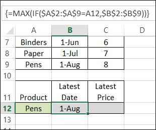
Last week, we used MAX and IF in an array-entered formula, to find the latest date that a product price was changed. Remember to press Ctrl + Shift + Enter after typing this formula, instead of just pressing Enter.

=MAX(IF($A$2:$A$9=A12,$B$2:$B$9))

Note: For more information on array formulas, I recommend Mike Girvin’s book, Ctrl+Shift+Enter: Mastering Excel Array Formulas.

Customers and Products

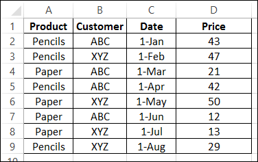
This week, our sample data has another column included – the customer name.

We’d like to revise that MAX and IF formula, to check for the latest date that a product price was changed, for a specific customer.

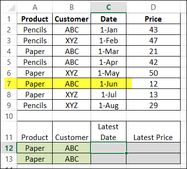
Select a Customer and Product

The product name, Paper, is entered in cell A12, and the customer name, ABC,  is in B2. By manually checking the list, we can see that the latest price change was on June 1st.

Modify the MAX and IF formula

The original formula just checked the product name, and then returned the latest date, from column B.

=MAX(IF($A$2:$A$9=A12,$B$2:$B$9))

Now, we want the formula to check both the product name (column A), and the customer name (column B), and return the latest date (column C).

Entered in cell C12, the formula will start the same, by checking the product name:

=MAX(IF($A$2:$A$9=A12,

Then we’ll add a second IF function, to check the customer name:

=MAX(IF($A$2:$A$9=A12,IF($B$2:$B$9=B12,

Finally, we’ll get the date from column C:

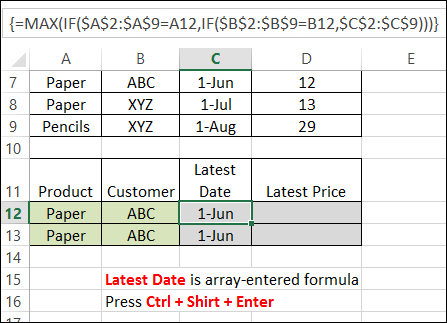
=MAX(IF($A$2:$A$9=A12, IF($B$2:$B$9=B12,$C$2:$C$9)))

IMPORTANT: After typing the formula, array-enter it, by pressing Ctrl + Shift + Enter.

The formula is copied down to cell C13, and both cells show the correct result – June 1st.

Get the Latest Price

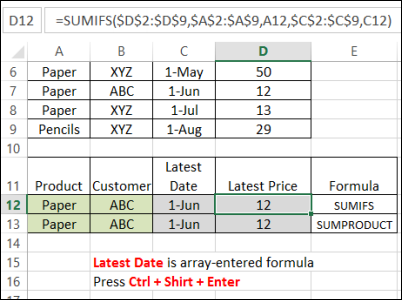
Finally, the Latest price is calculated using SUMIFS (Excel 2007 or later):

=SUMIFS($D$2:$D$9,$A$2:$A$9,A12,$C$2:$C$9,C12)

or SUMPRODUCT:

=SUMPRODUCT(($A$2:$A$9=A13)*($C$2:$C$9=C13)*($D$2:$D$9))

Download the Sample File

You can download the sample file from the MIN and MAX Functions page on my website.

• [Update]: In Excel 2019, and Excel for Office 365, you can use the new MINIFS and MAXIFS functions. There is more information on the MIN and MAX page on my Contextures site.

_____________________