
You can use the VLOOKUP function to find data in a lookup table, based on a specific value. If you enter a product number in an order form, you can use a VLOOKUP formula to find the matching product name or price. See how to use Excel VLOOKUP in different ranges.
NOTE: The examples below use VLOOKUP to get the value from the correct table. You could do a similar lookup with the INDEX and MATCH functions.
Two Lookup Tables
In some Excel workbooks, you might need to pull data from a specific table, depending on an option that the user has selected.
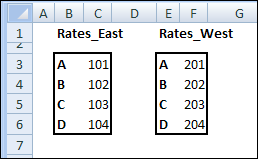
For example, in the screen shot below, there are different rate tables for the East and West regions.
- Range B3:C6 is named Rates_East
- Range E3:F6 is named Rates_West.
Create the VLOOKUP Formula
On the data entry sheet, if East is entered in column A, then the VLOOKUP formula should use Rates_East as the lookup table.
If West is entered as the region, the rate should come from the Rates_West table.

If there are only a couple of lookup tables, you could use an IF function to select the correct table in the VLOOKUP.
=VLOOKUP(B3,IF(A3=”East”,Rates_East,Rates_West),2,0)
This solution could work in this example, where there are only two rate tables.
Select the Correct Lookup Table
For situations when there are multiple lookup tables, an IF function probably wouldn’t be practical.
Instead, you can use the INDIRECT function to return the correct lookup range.
=VLOOKUP(B3,INDIRECT(“Rates_” & A3),2,0)

The INDIRECT function combines the text string “Rates_” with the region entered in column A, and returns the range with that name.
In the screen shot above, “West” was entered as the Region in cell A3. The VLOOKUP formula will use Rates_West as the lookup table, and return the value for Group C in that table.
Using the INDIRECT function with named ranges makes the VLOOKUP formula very flexible, and you could use any number of lookup tables in the workbook.
______________
Debra – Based on what i recently learned, I would tend to use a combination of the index and match functions instead. For example, if the database had columns labeled Group, East and West in Columns A, B and C respectively (no named ranges), in a sheet named “Rates,” the formula in Cell C3 in your last example would be =INDEX(Rates!$A$1:$C$5,MATCH(B3,Rates!$A$1:$A$5,0),MATCH(A3,Rates!$A$1:$C$1,0)). Hope this is helpful. Bob
Thanks Bob, I have an example like that on my INDEX/MATCH page:
http://www.contextures.com/xlFunctions03.html#IndexMatch2
The goal in this blog post was to select a specific table for the lookup, and you could use the same technique within an INDEX/MATCH formula.
In my real-life workbook, there’s a rate table for each of 12 regions, and each table is about 20 columns wide and 100 rows tall. Based on the region selected, the correct rate table has to be used.
Hi Debra,
One thing for the user to watch out in this solution is the fact that INDIRECT() is volatile, so if the tables are big enough and the number of formula instances is reasonably high the recalculation might become annoying. One way around, assuming all tables are on the same sheet, could be:
=VLOOKUP(B3,INDEX((Rates_East,Rates_West),,,MATCH(A3,{“Rates_East”,”Rates_West”})),2,0)
If there are a few tables you could define 2 named formulas, e.g.:
Tables=Tables!$B$3:$C$6,Tables!$E$3:$F$6,Tables!$H$3:$I$6,Tables!$K$3:$L$6
NamesList={“East”,”West”,”South”,”North”} ‘could also come from a range of cells
and then use them in the final formuala as follows:
=VLOOKUP(B3,INDEX(Tables,,,MATCH(A3,NamesList)),2,0)
Also, if you use VLOOKUP() to retrieve information from n columns, you are repeating the search n times. The advantage of MATCH() is you can isolate the search in an anchor cell and reference it n times without recalculating it. For example:
Tables=Tables!$B$3:$D$6,Tables!$F$3:$H$6,Tables!$J$3:$L$6,Tables!$N$3:$P$6
NamesList={“East”,”West”,”South”,”North”} ‘could also come from a range of cells
[C3]=MATCH($A3,NamesList,0) ‘table index
[D3]=MATCH($B3,INDEX(Tables,,1,$C3),0) ‘row index
[E3]=INDEX(Tables,$D3,2,$C3) ‘data from the 2nd column
[F3]=INDEX(Tables,$D3,3,$C3) ‘data from the 3rd column
Thanks KL, that’s great advice and excellent suggestions for alternate formulas.
Hi Debra,
I am using a if statement with a vlookup and an indirect set of lists. I got it to work with one name “CCC1- Call” but when I try to add another name, “CCC2- Contact” it won’t work. What am I doing wrong or missing. Here is the formula I am using in the Data Validation source box: =IF(or(C6=”CCC1- Call”,INDIRECT(VLOOKUP(C8,Namelookup2,2,0,IF(C6=”CCC2- Contact”,INDIRECT(VLOOKUP(C8,Namelookup5,2,0)))))))
How do I also bring over the cell comment when I do a vlookup?