
Now that the 30 Excel Functions in 30 Days challenge has ended, it’s time to look at a few other features. On the Contextures page on Facebook, Lee suggested AutoFilters as a topic for some February posts. Thanks Lee! Here’s how to turn off filters in Excel table headings.
Category: Excel Filter
Excel AutoFilter With Criteria in a Range
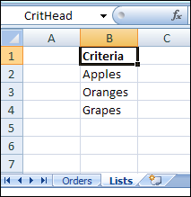
In Excel 2003, and earlier versions, an AutoFilter allows only two criteria for each column. In Excel 2007 and later, you can select multiple criteria from each column in the table. See how to apply an Excel AutoFilter with multiple criteria in a range on the worksheet.
Update: Get the latest version of this workbook on my Contextures site: Filter Criteria List Macro.
Continue reading “Excel AutoFilter With Criteria in a Range”
Excel 2007 AutoFilter Dynamic Dates
 Over on the Contextures website, I’ve updated the AutoFilter Intro page, so it now covers the basics for Excel 2007 AutoFilters.
However, many people are still using an older version of Excel, so I’ve moved the original material to the Excel 2003 AutoFilter Basics page.
Improvements in AutoFilters
AutoFilters are easier to use in Excel 2007 and Excel 2010, and the filter and sort options are automatically added in the top row, if you format your list as an Excel Table.
Filter for Dynamic Date Ranges
Among the new AutoFilter features that were introduced in Excel 2007 are dynamic date ranges.
A Dynamic Date Range is one that changes automatically, as time moves forward.
For example, you could select Yesterday, which will represent a different date, every day that you open the Excel file.

Update Filters
Unfortunately, the dynamic dates are only semi-dynamic, and they don’t magically change when you open the workbook at a later date. You’ll need to update the filter to see the current information.
You can update the Excel 2007 AutoFilter manually, by clicking Reapply on the Excel Ribbon. Or, you could add a bit of code to the Workbook_Open event, to reapply the filters automatically.

Learn More About Excel 2007 AutoFilters
If you’re not familiar with the new features in Excel 2007 and Excel 2010 AutoFilters, you can learn more at Excel 2007 AutoFilter Basics.
_____________
Excel Advanced Filter Painfully Slow
Today, working on my Excel file was like riding a lazy snail through molasses in January — but slower!
Usually an Excel Advanced Filter is a speedy way to extract data from a table, but things weren’t working right in a sample file that I got last week.
And despite what my high school English teachers might think, you can’t mix too many similes, when trying to describe excruciating slowness.
Advanced Filter Macro Problem
The sample file had code that ran an Advanced Filter in Excel 2007.
The code ran quickly in Excel 2003, but screeched to a near halt in Excel 2007. What was the problem?
In the sections below, I detailed all the things I tried, while troubleshooting the slow macro problem.
- Tip: You can skip to the end, to see what the unexpected problem was, and how I finally fixed the Advanced Filter macro.
There’s a video at the end of this post too, where I show the problem and the solution.
The Slow Filter Symptoms
When the code ran in Excel 2007, it looked like the extracted rows were being pasted in the second worksheet, one row at a time.
Aha! I should turn off the screen updating — a simple solution. You’d think.
Nope! Even with the screen updating turned off, the code barely crawled along.
It took almost 3 minutes to extract 1500 rows — maybe a millisecond faster than it ran with screen updating turned on. Who has that kind of time?
Guess Again
In the next round of solution guessing, I got rid of the few formulas in the worksheet and criteria range.
There wasn’t anything too complex, but maybe that was slowing things down.
I also changed calculation to manual at the start of the code, then set it to automatic at the end of the code.
Neither of those changes had any effect on the code’s speed.
Strip the Data Clean
In round 12 of testing (I’ve lost track of the test count), I copied the data, and pasted it as values into a new workbook.
The code ran like lightning. In July. With jet engines. Hmmm.
Maybe it was the formatting and styles in the original file that were slowing things down.
To test that theory, I formatted the original table with Normal style, which removed all the borders and fill colour.
That didn’t improve things, but when I removed the red fill from the heading cells, I noticed a red comment marker in one of the cells.
Whip Things Into Shape
Could a comment be the problem? That didn’t seem likely, but:
- As soon as I deleted the comment, the code ran perfectly.
- When I put the comment back, the macro slowed to a crawl again.

Curiouser and Curiouser
When I tried to create a sample file to demonstrate this problem, things got even stranger.
I created a table with a comment in the heading, and ran the code, expecting it to be slow. It ran quickly, in several tests.

Add Shape to Worksheet
Next, I added a shape to the worksheet, and assigned a macro, to make it easier to run the code.
The code slowed down again!

Next, I deleted the shape, and the code was still slow, so I had to delete the comment to speed it up again.
The Verdict on Slow Advanced Filter Macro
If your Advanced Filters are running slowly in Excel 2007, try removing any comments in the table heading cells.
You could delete them at the start of a VBA procedure, run the filter, then add the comments at the end of the code.
Shapes + Comments = Trouble
The problem seems to occur if there are heading comments, and a shape is added later, as you can see in the short video demonstration below.
Fortunately, this problem appears to be fixed in Excel 2010, so if you upgrade, you should be able to have comments and shapes, without slowing down the Advanced Filters.
Another Solution
Update: In the comments, PDLobster suggests the following solution, to speed up the filters — thanks!
- Turn off all filters
- Select cell A1
- Turn Wrap Text ON
- Select the entire worksheet
- Turn Wrap Text OFF
Watch the Video
To see the steps for reproducing and solving the Advanced Filter speed problem, you can watch this short Excel video.
____________
Add Filter Markers in Excel Pivot Table
If you’re using Excel 2007 or Excel 2010, you can quickly see which fields in a pivot table have filters applied.
For example, in the screenshot below, the ItemSold field has been filtered.
The arrow drop down has changed to a filter symbol, with a tiny arrow.

Earlier Excel Versions
In Excel 2003 though, there’s no indicator that a field has been filtered. Here’s the same filtered pivot table in Excel 2003, and the drop down arrows look the same in both of the fields.
There’s no marker to show if either field has been filtered. You’d have to click each arrow, to see if any of the check marks have been removed from the pivot items. Who has time for that?

Create Your Own Filter Markers
Several of my clients are still using Excel 2003, and maybe you use it too. If so, you’ll appreciate this sample Excel file from AlexJ, which adds a bright blue marker above each filtered field.
That makes it easy to keep track of what’s been changed in the pivot table, and prevents you from overlooking the filters.
- Tip: You could even use these markers in newer versions of Excel. The bright blue arrows are easier to see than the tiny filter icons!

User Defined Function
To create the markers, Alex wrote a user defined function, named pvtFilterID.
In the screenshot below, you can see the pvtFilterID formula in cell D5, which refers to the ItemSold field heading in cell D7.
=pvtFilterID(D$7)
The formula is used in cells B5:D5, above the row fields, and that range could be adjusted if your pivot table has a different number of row fields.

The Blue Arrow Marker
Cell D1 is named Symbol.Filter, and it contains the blue arrow symbol that’s used as a marker.
If you changed the symbol there, the new symbol would be used as the filter marker.
In cell G5 there’s another formula, that shows a message if any of the pivot table fields are filtered.
- =IF(COUNTIF($B$5:$D$5,Symbol.Filter)>0, “Pivot Filter On” & Symbol.Filter,””)
This formula checks the cells above the pivot table, and shows the message if any of those cells contain the marker symbol.
Works With Slicers Too
Even though Alex wrote this code for Excel 2003 pivot tables, it works in Excel 2007 and Excel 2010 too.
In the screenshot below, you can see and Excel 2010 pivot table with slicers, and the filter markers highlight the row fields where filters have been applied.
The filter symbol is on the field drop downs too, and the bright blue markers are extra insurance that users notice which fields are filtered.

The Filter Marker Function Code
Here’s Alex’s code for the pvtFilterID function.
Function pvtFilterID(rng As Range) As String  'rng As Range)
On Error GoTo XIT ' -not in pivot
If Not rng.Parent Is ActiveSheet Then GoTo XIT
If rng.Cells.Count > 1 Then
    MsgBox "Error: pvtFilterID range selection"
    GoTo XIT
End If
If rng.PivotField.HiddenItems.Count > 0 Then
    pvtFilterID = [Symbol.Filter]
End If
XIT:
End Function
Clear the Pivot Table Filters
Another nice feature that was added to Excel 2007 pivot tables is the Clear All Filters command. Alex’s workbook contains a button that runs code to remove all the filters from a pivot table.
Here’s the code for the ClearPivotFilters procedure.
Sub ClearPivotFilters(ws As Worksheet)
    Dim pvt As PivotTable
    Dim pf As PivotField
    Dim pi As PivotItem
    Dim lSort As Long
On Error Resume Next
Set pvt = ws.PivotTables("PivotTable1")
For Each pf In pvt.VisibleFields
    If pf.HiddenItems.Count > 0 Then
      lSort = pf.AutoSortOrder
      pf.AutoSort xlManual, pf.SourceName
      For Each pi In pf.PivotItems
        pi.Visible = True
      Next pi
    End If
    pf.AutoSort lSort, pf.SourceName
Next pf
Set pi = Nothing
Set pf = Nothing
Set pvt = Nothing
End Sub
The button code passes the worksheet name to the procedure.
Private Sub cmdClearPvtFilters_Click()
    Call ClearPivotFilters(Me)
End Sub
Download the Sample File
To test the pivot table filter markers, and see the VBA code, you can download Alex’s sample file from the Contextures website.
On the AlexJ Sample Files page, go to the Pivot Tables section, and look for: PT0000 – Pivot Table Filter Markers
___________
Excel Slicers for Easy Pivot Table Filtering
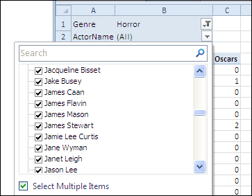
Slasher movies are a scary Halloween tradition, and you can fight back against these horror films, by using Excel Slicers to slash through piles of data.
The Guardian recently posted a list of Greatest Films of All Time. Let’s see how we can use Excel Slicers for Halloween horror films from that list.
Continue reading “Excel Slicers for Easy Pivot Table Filtering”
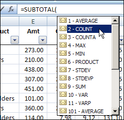
Count Unique Items in Excel Filtered List
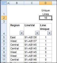
You can use the SUBTOTAL function to count visible items in a filtered list. In today’s example, AlexJ shows how to count the unique visible items in a filtered list. So, if an item appears more than once in the filtered results, it would only be counted once. Thanks, AlexJ!
Continue reading “Count Unique Items in Excel Filtered List”
New Search Feature in Excel 2010 AutoFilter
Last week, you saw a quick tip for filtering by selection in Excel 2007. That’s helpful when you’ve found an item in a list, and want to filter for that item.
There’s another new feature in the AutoFilter dropdown, in Excel 2010.
When you click the drop down arrow in the AutoFilter heading cell, you’ll see a new Search box, that wasn’t in previous versions of Excel.

This is a great way to find an item in a really long list — much quicker than scrolling down, and scanning all the list items.
Use the Search Box
For example, if you type “ri” in the Search box, only the cities with “ri” in their name will be left in the drop down list.
In the screen shot below, “riv” is in the Search box, and only one city (Riverview) is showing — the only city with that string of letters in its name.

Press the Enter key to complete the search, and the worksheet is filtered for the selected city names.

Watch the Video
To see the steps in the AutoFilter Search, you can watch this short Excel tutorial video.
____________
Filter for Selected Item in Excel List
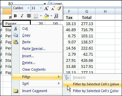
Last month you saw a quick way to filter for the selected item in a pivot table, and today you’ll see a similar technique for a worksheet list in Excel 2007.
Tip: For the Excel 2003 quick filter instructions see AutoFilter By Selection in Excel
Number Visible Rows in Excel AutoFilter
When you create a list in Excel, do you start with a column that numbers the rows? I usually create an ID column and type the number, or use a formula to automatically number them.

In the steps below, I’ll show you the simple numbering system. There’s a fancier formula too, if you’d like to see consecutive numbers when the list is filtered.
