I included some movies from the Top 250 Movies list at the IMDb website. You can add movies from your DVD collection, or your Netflix list.
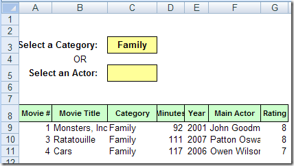
Then use the selection boxes to see movies from a specific category, and/or featuring your favourite actor.
In the previous version, you could only choose Category OR Actor, and now you can choose one or both. (Exciting, I know!)
Or, clear both criteria cells, to see all the movies.
Select a movie category
Download the Sample File
You can download the Excel movies database file from the Contextures website. It’s in Excel 2003 format, and zipped.
The file contains macros, so you’ll have to enable those to make the file work.
The Perfect Computer
I couldn’t find any movies about Excel, to add to the Excel movies database, but computers play a leading role in several movies. You might remember HAL 9000, from “2001: A Space Odyssey”.
HAL: Let me put it this way, Mr. Amor. The 9000 series is the most reliable computer ever made. No 9000 computer has ever made a mistake or distorted information. We are all, by any practical definition of the words, foolproof and incapable of error.
Yes, that was the dream, way back in 1968, when they made “2001: A Space Odyssey”. Over 40 years later, we haven’t even come close to achieving that goal! Well, maybe it’s not the computers’ fault – the users might be part of the problem.
Random Draw Sinner
Congratulations to Alex Kerin, whose name I selected in the random draw for the Excelerator Quiz giveaway. Here’s his name at the top of the list, after I used the RAND function, and sorted the Rand column in ascending order.
Alex’s prize is a 23″ monitor, plus a keyboard and mouse, courtesy of the PowerPivot team. Thanks to everyone who participated, and to the PowerPivot team, and Megan at Ignite Social Media, who organized the giveaway.
It’s Price Book publishing week for one of my clients, and we’ve been making lists, and checking them twice. Or 3 or 4 times, or more!
When comparing the new prices to the previous prices, an Excel AutoFilter comes in handy. You can select the same product or model in each workbook, and easily compare item details.
Yes, the widget prices went up a bit this year, so that’s why the assembled parts cost a bit more.
There are written steps and a video below, that show how to use the AutoFilter feature, and workarounds for a problem
Record Count in the Status Bar
Sometimes when you select records with an AutoFilter, the record count appears in the Status Bar, at the bottom left. In this example, I was working with a small table, with 50 records, and only one column had a formula.
I selected File Folder in the Product column, and the Status Bar showed that 3 of the 50 records contained that product. So far, so good.
Record Count in the Status Bar
Status Bar Shows Filter Mode
Then I added another record to the table, and selected a different product from the AutoFilter drop down list. This time the Status Bar showed the rather unhelpful message, “Filter Mode”, instead of the record count.
Excel 2007 seems to handle this better, but in Excel 2003, and earlier versions, you might see “Filter Mode” if there are more than 50 formulas in the list.
When you apply an AutoFilter, the formula recalculate. If there are lots of formulas to calculate, Excel shows a “Calculating %” message in the Status Bar, so you’ll have something to entertain you while you wait.
Unfortunately, the “Calculating %” message interferes with the record count message in the Status Bar. If the record count message is interrupted, it shows the “Filter Mode” message instead.
You can’t change this behaviour, but there are a couple of workarounds that you can use to find the record count.
Use AutoCalc Instead
If the Status Bar shows “Filter Mode”, you can get the record count from the AutoCalc feature instead.
Right-click on the Status Bar
In the pop-up menu, click Count Nums
Click on the column heading for a column that contains numbers (and no blank cells within the list)
You’ll see the count of visible numbers in the AutoCalc area of the Status Bar.
AutoCalc area of Status Bar
Use the SUBTOTAL Function
If you’d rather have the record count show up automatically, you can use the SUBTOTAL function. It ignores the filtered rows, and calculates based on the visible rows only.
For example, with numbers in column D, this formula, with 2 as the first argument, will calculate the COUNT of visible numbers:
=SUBTOTAL(2,D:D)
Use the SUBTOTAL Function
If you want to count items in a column that contains text, use 3 as the first argument, and subtract 1 from the result, to account for the heading cell.
=SUBTOTAL(3,B:B)-1
Watch the Excel AutoFilter Video
In this very short video you can see my Excel AutoFilter experiment, and watch the Filter Mode message appear in the Status Bar.
There are no ruggedly handsome math teachers in this video, but it’s fun-filled and action-packed!
In Excel 2003 and earlier versions, you can use an Advanced Filter to remove duplicates. In Excel 2007, there’s a new command on the Ribbon to make it easier to remove duplicates from a list.
Be careful with the Excel 2007 Remove Duplicates feature though – it really removes the duplicates. If you use an Advanced Filter instead, you have the option of hiding duplicates, or creating a unique list in a new location.
How It Works
Update: Jason Morin asked a few questions about the Remove Duplicates feature, and how it works, so I’ll answer the questions here. (Thanks Jason!)
1) Does the new Duplicates capability discern between text strings and numerical values that look the same on the screen?
No, it treats the text strings and numbers the same. If the list has a 10 and a ’10, they’ll be treated as duplicates. There isn’t a settings option that I can see, where you can adjust this. In the Advanced Filter feature, those would be seen as 2 unique items.
2) What about non-visible characters in the cell? Does it consider “Pen” and “Pen ” the same? As a user I would view this as a duplicate, but Excel may not.
No, those won’t be treated as duplicates, because the space character in the second entry makes it different. Advanced Filter would do the same.
3) How does it decide WHICH duplicate to remove in the data set?
The first instance of each item is left, and all subsequent entries are deleted.
4) I assume if I’m working with record set (>1 column), I need to concatenate data from columns to create a unique identifier for each record, then run the Duplicates on the new column I created.
You can use the check marks in the Remove Duplicates dialog box, and select all the columns you want to include. Only if all the included columns are duplicated, will an item be removed. Advanced Filter works the same way, but without the check marks.
Remove Duplicates
In this example, the list in cells A1:A10 contains a few duplicates.
Follow these steps to remove the duplicates.
Select any cell in the list, or select the entire list
On the Ribbon’s Data tab, click Remove Duplicates.
In the Remove Duplicates dialog box, select the column(s) that you want to remove duplicates from
Check the box for My Data Has Headers, if applicable, then click OK.
Remove Duplicates dialog box
A confirmation message will appear, showing the number of duplicates removed, and the number of unique items remaining. Click OK to close the message.
Watch the Remove Duplicates Video
Here’s a very short video that shows the steps to remove duplicates in Excel 2007.
I know about those problems, and am careful to avoid them.
A Simple Filter
This week, as part of a larger procedure, I had an advanced filter, similar to the one shown below.
Filter for Unique Products
The code was designed to pull a list of unique products from column G, and put it in column K.
In this example, all 7 products in column G are unique, so they all should have been filtered to column K.
However, after I ran the filter, there was nothing in column K, except the heading!
Leftovers Clog the Filter
I checked, and the headings were an exact match, so that wasn’t the problem.
I checked the code carefully, and everything looked okay. Similar code had run hundreds of times, without a hiccup.
To troubleshoot, I tried to run the advanced filter manually, and in the screen shot below, you can see what appeared in the Advanced Filter dialog box when it opened.
Hmmm. There, in the Criteria Range box, was the range from a previous advanced filter.
Clear Criteria Range Setting
I cleared out the Criteria Range setting, and the filter ran without problems.
As expected, all 7 products showed up in column K.
Change Advanced Filter Macro Code
To prevent the macro problem from happening again in the future, I revised the macro code.
Even though the advanced filter didn’t use a criteria range, I added one to the code, with the setting as an empty string.
Good Housekeeping Prevents Clogging
With that change, the code ran perfectly, even if a previous filter had a criteria range.
To prevent your own advanced filter headaches, add that empty criteria range to your code, if you’re not using a criteria range.
It will clear out the setting, in case a previous advanced filter used a criteria range.
I’ll certainly do that from now on!
__________________
For a simple database, Excel can do a pretty good job of organizing and reporting your data. This example shows a movie collection database in Excel, but you could set up something similar to keep track of books, sales orders, or almost anything else.
In the steps below, I’ll show how to set up an Excel workbook so you can click on a map, and see a list of fictional doctors in the state that you selected. There’s also an Excel sample file that you can download, and try this map technique for yourself!
Click state on map to get list of fictional doctors
Set up the Map
First, I found a clip art map of the continental USA, with a separate shape for each state, and pasted that into a workbook.
Next, I named the shapes, using the two digit state abbreviation.
Click on a state shape, e.g. Washington
Click in the Name Box, and type the two digit code – WA
Map of USA with state shapes
Press the Enter key, to complete the naming.
This will be a good test of your geography knowledge and state abbreviation skills.
Set Up the List of Doctors
On a sheet named Doctors, I entered a list of fictional doctor names, state codes and number of patients.
The macro. named GetDoctorList, uses an Advanced Filter, to extract a list of doctors for the selected state.
Sub GetDoctorList()
On Error Resume Next
Dim strState As String
Dim sh As Shape
Dim wsMap As Worksheet
Dim wsDoctor As Worksheet
Dim wsList As Worksheet
strState = Application.Caller
Set wsMap = Worksheets("Map")
Set wsDoctor = Worksheets("Doctors")
wsMap.Range("A2").Value = strState
wsDoctor.Range("DoctorList").AdvancedFilter _
  Action:=xlFilterCopy, _
  CriteriaRange:=wsMap.Range("Criteria"), _
  CopyToRange:=wsMap.Range("StateList"), Unique:=False
wsMap.Activate
wsMap.Range("A1").Activate
End Sub
Assign the Macro to Shapes
The final step is to assign the GetDoctorList macro to each State shape in the USA map.
You could do this manually, if there were just a few shapes:
Right-click on each shape
Click the Assign Macro command
Select the GetDoctorList macro
Click OK
Macro to Assign Macros
It might take quite a while to assign the GetDoctorList macro for all 48 states!
So, I wrote another macro, to do the work for me.
You’ll only have to run this macro once, while setting up the workbook.
The macro is only a few lines long, and it assigns the GetDoctorList macro to each shape on the worksheet named Map.
Sub AddMacro()
Dim sh As Shape
For Each sh In Worksheets("Map").Shapes
    sh.OnAction = "GetDoctorList"
Next
End Sub
Run the Filter
Now, to run the filter, you can click on a state in the map.
When the GetDoctorList macro runs, it does the following steps:
First, it puts the state code in cell A2
Next, the macro runs an advanced filter, which puts the list of doctors in the extract range, starting in cell B18.
The criteria range, and the extracted list are shown in the screen shot below.
The state shape for California (CA) was clicked, and the filtered list shows the fictional doctors from California.
click on a state in the map
Get the Sample File
To get the Excel sample file with the USA map and list of fictional doctors, go to the Excel Filter Sample Files page on my Contextures site.
On that page, go to the section named: Filter Files FL0011 – FL0020
In that section, look for the sample file named FL0012 – Map Based Filter, and click its download link.
The zipped Excel contains macros, so be sure to enable those, if you want to test the map filter macros.
The same feature is available in Excel 2007, using a different technique.
Excel Worksheet List
Using the same example as in the previous post, the East region is selected in the table below.
With a couple of clicks, and no programming, you can add an AutoFilter and filter the table to show only the East region orders.
Excel Worksheet List
Apply the AutoFilter
In previous versions of Excel, you had to add a toolbar button to use the filter by selection feature.
In Excel 2007, the feature is available in a shortcut menu.
The table doesn’t need to have an AutoFilter currently applied.
In a table in Excel, right-click a cell that contains the criterion you’d like to use. For example, to filter for the East region records, right-click an East cell in the Region column.
On the shortcut menu, click Filter, then click Filter by Selected Cell’s Value
An AutoFilter is added to the table, if there wasn’t already one in place. The table is filtered, and shows only the East region records.
Remove the Filter
To remove the filter, and show all the records again:
In the Region column heading, click the AutoFilter drop down arrow
Click Clear Filter From “Region”.
Clear an Excel AutoFilter
The filter is removed from the Region column, but the AutoFilter feature is still turned on.
In related news, I recently discovered that the mouse shortcut to copy and paste as values doesn’t work anywhere on a filtered sheet, unless all the records are showing.
Here you can see that it’s not available on the shortcut menu.
Use Ribbon Command
You can use other methods to copy and paste as values, such as the Ribbon command, but not the shortcut. I wonder why.
In Excel 2003, you can add a couple of buttons to the toolbar to make it easy to filter a table.
For example, in the table below, the East region is selected. With one click of a button, and no programming, you can add an AutoFilter and filter the table to show only the East region orders. Thanks to Roger Govier for sharing this tip.
In Excel, you might have a long list of orders with a grand total at the end. If you filter the Region column, so the list only shows one region’s sales, you’d like the total to include only those items. Here’s how to total a filtered list in Excel.