
Microsoft just announced the winner of their Excel World Champ data visualization contest. Congratulations to Ghazanfar Abidi, from Canada! I found his website today, and learned something new from his latest blog post – depending on how you apply it, pivot table fill colour might disappear!
Combine VLOOKUP and MATCH for Flexible Formula
With the Excel VLOOKUP function, you can pull data from a specific column in a lookup table. For example, if the lookup table has Product ID, Product Name and Price, you’d use column 3 to get the price. To make your formulas more flexible, and to prevent problems, you can combine VLOOKUP and MATCH.
Continue reading “Combine VLOOKUP and MATCH for Flexible Formula”
Take the Excel Name Fix Challenge
Last week, in my Contextures Newsletter, I posted an Excel Name Fix challenge. There was a short list of names, which needed to be fixed. Then we needed to count how many were fixed. Take the challenge yourself – download the workbook to see how you’d solve it.
Freeze All Worksheets Macro
If you’re working with a large worksheet in Excel, it usually helps if you freeze the cells at the top and/or the left side of the sheet. That way, your headings are always visible, along with other key information that you’ve put at the top of the sheet. You can freeze each sheet individually, or use this macro to freeze all worksheets at once.
Fix Excel Conditional Formatting Duplicate Rules
Conditional formatting is a great way to highlight specific data, but did you know that it can automatically create new rules on its own? I’ll show you how that happens, and an easy way to fix those conditional formatting duplicated rules.
Continue reading “Fix Excel Conditional Formatting Duplicate Rules”
Excel RANK IF Formula Example
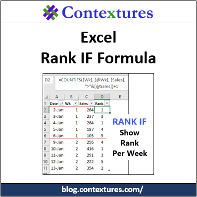
There is a Microsoft Excel RANK function, so you can calculate where each number stands in a list of numbers. There isn’t a RANKIF function though, if you need to rank based on criteria. Someone asked me for help with ranking daily sales, so I used COUNTIFS to make an Excel Rank If formula workaround.
Popup List of Excel Sheets
If you’re working in an Excel file with lots of worksheets, it can take a while to scroll to the ones that you need. Sometimes you can’t even remember where the sheets are, and that takes even longer! To make it easier for myself, I created an add-in with a popup list of Excel sheets. See the details below, and there’s a link to my site where you can download it.
Impressive Dashboards with Google Sheets
Over the years, I’ve used Google Sheets a few times, and usually for basic tasks. Yesterday, I was surprised and impressed to see what it can do, thanks to Ben Collins. He builds interactive dashboards with Google Sheets, complete with pivot tables and maps, using the built-in features. Who knew that all this was possible, in a free, online spreadsheet application?
Pivot Table Subtotal Problem in Excel 2016
If you using grouping, you might run into a pivot table subtotal problem in Excel 2016. There was a change in a recent update, so you might see this problem if you have an Office 365 subscription. I just learned about this issue, and will show you how to fix the problem if it affects your workbooks.
Continue reading “Pivot Table Subtotal Problem in Excel 2016”
Excel VLOOKUP Problem Numbers
Recently, someone asked me for help with VLOOKUP problem numbers:
- He had a list of 8-digit numbers.
- In the next column, there was a formula to get the first 3 numbers: =LEFT(A2,3)
- Based on that number, a VLOOKUP formula should find the category in a lookup table
- Problem – Instead of a category name, the result is an #N/A error.
The VLOOKUP formula looks okay, so why doesn’t it work?