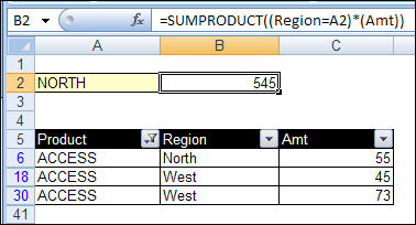
Last week, we used the Excel SUBTOTAL function to sum items in a filtered list, while ignoring the hidden rows. Now we’ll look at ways to use Subtotal and SumProduct with filter settings applied.
One of my clients uses a pivot table to summarize product sales, using sales data from their accounting system. Occasionally, they’d like to type a number in the pivot table, but Excel won’t let you change values in a pivot table. Here is a workaround for that limitation.
Long ago, when many of the pivot table features were hidden away in obscure menu and dialog boxes, I created the PivotPower add-in. It makes it easy to do pivot table tasks, such as:
change the summary function for all the data fields from Count to Sum,
reset the field captions,
protect the pivot table layout,
and many other tasks
When you install PivotPower, it adds a a drop down list on the Add-ins tab of the Excel Ribbon, or a menu on the menu bar, in older versions of Excel.
Latest PivotPower Update
In the latest version of PivotPower, most of the commands will only affect the selected pivot table.
For example, if there are two pivot tables on the worksheet, select a cell in one pivot table, before using the COUNT All Data command. The data fields in the selected pivot table will change.
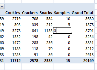
If the active cell is not in a pivot table, all pivot tables on the active sheet will be affected when you run the command. In the screen shot below, a cell between the pivot tables is selected.
When the SUM All Data command is selected, both pivot tables will be changed.
PivotPower Fix
This version of PivotPower also has a fix. In the previous version, if you selected the AVERAGE All Data command, the Data labels changed, and stayed as “Avg” even if you selected a different summary function.
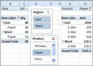
In Excel 2007, and earlier versions, you can use Excel VBA code if you want to automatically filter multiple pivot tables at the same time. That task is much easier in Excel 2010, thanks to the new Slicer feature.
ISREF and the IS Functions — although it sounds like the name of a geeky band, it’s not. Today we’ll take a look at ISREF, which is one of the 9 IS functions that are lumped together in the Excel Help files.
How sad — 9 functions that never get to shine on their own. We’ll give ISREF a few minutes in the spotlight, to see how it works.
The Excel IS Functions
The following IS functions are listed on one page in Excel Help:
ISBLANK(value)
ISERR(value)
ISERROR(value)
ISLOGICAL(value)
ISNA(value)
ISNONTEXT(value)
ISNUMBER(value)
ISREF(value)
ISTEXT(value)
They all work in the same way — the function tests a value, and returns TRUE if the value passes the test.
NOTE: There is also a new ISFORMULA function for Excel 2013 and later versions.
IS Function Examples
For example, if cell B2 contains a number, the ISNUMBER formula will result in TRUE:
=ISNUMBER(B2)
ISNONTEXT Function Excample
If cell B3 contains anything except text, even if cell B3 is blank, the ISNONTEXT formula will result in TRUE:
=ISNONTEXT(B3)
ISNONTEXT Function Example
The other IS functions work the same way, and give the expected results — except for ISREF.
ISREF Function Problems
In the screen shot below, there is a reference in cell B2, with the following formula: =D1
In cell D2, the ISREF function returns TRUE as the result.
However, the ISREF function also returns TRUE in cell D3, even though there is a typed value in cell B3 — the number 7
How ISREF Function Works
The ISREF function isn’t testing what’s in the referenced cell, it’s testing the reference within the formula.
And because the ISREF formulas in both D2 and D3 contain references, the result is TRUE for both formulas.
So, the ISREF function won’t help you assess whether there is a reference another cell.
ISREF Uses
If you can’t use ISREF to detect a reference in another cell, how can you use it?
Well, ISREF can check the results of other formulas, to see if they have returned a valid reference.
You could use ISREF, instead of ISERROR, in your formulas that need references.
For example, in the screen shot below, the INDIRECT function in cell D2 returns a reference, and INDIRECT(“D1”) creates a valid reference.
If cell B2 contains the text “D1”, this formula results in TRUE:
=ISREF(INDIRECT(B2))
ISREF With OFFSET
The first OFFSET formula in the screen shot below is not valid, because there is no cell that is 1 column to the left of cell A1, so the ISREF result is FALSE
=ISREF(OFFSET(A1,0,-1))
Hoever, the second OFFSET formulas returns a valid reference to cell B1, so the ISREF result is TRUE.
Any Other Uses for ISREF Function?
Do you use ISREF in your formulas? Can you think of any other examples for using it?
______________ Save
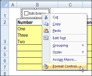
A couple of years ago, I described how you could select multiple items from an Excel drop down list. One of my clients needed that feature in a workbook last week, so I’ve made an enhancement to the VBA code. Now you can edit multiple selections in Excel after entering them.