Excel UserForm Data Entry Update

Someone emailed me this week, about a problem he was having with my sample Part Data Entry UserForm.

PartsInventoryUserForm01

When I took a look at the workbook, everything seemed okay, and the code had been copied and altered correctly.
Excel Named Table

Then I noticed that there was a formatted Excel table on the data collection sheet, which wasn’t in my original file.

That can cause problems if you’re using Excel VBA to add data to the first blank row on the worksheet.

Change the Last Row Code

In the comments for my Find First Blank Row blog post, Rick Rothstein suggested this code revision:

LastRow = Cells.Find(What:="*", SearchOrder:=xlRows, 
SearchDirection:=xlPrevious, LookIn:=xlValues).Row

Rick mentioned that this formula ignores cells with formulas that are displaying the empty string. If your situation is such that you need to identify formula cells that might be displaying the empty string, then change the xlValues argument to xlFormulas.

Revised Excel VBA Code

So, I changed the Part Data Entry code, to use the Find method for finding the last row. I replaced this old line of code:

'find first empty row in database
iRow = ws.Cells(Rows.Count, 1) _
  .End(xlUp).Offset(1, 0).Row

With this line of code:

iRow = ws.Cells.Find(What:="*", SearchOrder:=xlRows, _
       SearchDirection:=xlPrevious, LookIn:=xlValues).Row + 1

Parts Data Entry UserForm With Combo Boxes

There is another version of the Parts Data Entry UserForm, and it’s a little fancier, with combo boxes to select parts and locations.

I’ve updated the Parts Data Entry UserForm With Combo Boxes too, with the revised last row code.

PartsInventoryUserForm02

Get the Updated Sample Files

You can download the updated versions of the parts data entry forms on the Contextures website.

Part Data Entry UserForm

Parts Data Entry UserForm With Combo Boxes

_________________

Updated Excel Weight Loss Tracker

You know how tough it can be to maintain two versions of the same file. It creates twice as much work for you, and no extra rewards! So, instead of having two versions of the Excel weight loss tracker – pounds and kilograms – I’ve rolled them into one workbook.

For now, there is a separate file for the stone measurements, because it has a different layout on the data entry sheet. If possible, I’ll roll that version in later.

Continue reading “Updated Excel Weight Loss Tracker”

Excel Drop Down From List in Different Workbook

To make it easier for people to enter data, you can create drop down lists on an Excel worksheet.

Usually the source lists are stored in the same workbook as the drop downs. However, with named ranges, it is possible to use a list in a different workbook.

In the screen shot shown below, the original list is in the workbook at the left. The drop downs are in a different workbook, on the right.

DataValListLinked

There Is a Catch

My preference would be to keep the lists and drop downs in the same workbook, but if you need to have them in separate files, this technique will allow you to do that.

There’s one catch though, when using this data validation technique. The source workbook, which contains the original list, must also be open, when you are using the drop down lists.

So, it’s not a perfect solution, but it’s fairly easy to implement, as long as you remember to open the other workbook too.

Excel 2010 Instructions

I’ve just uploaded a video with instructions for this technique in Excel 2010, so you can see the steps for creating the named ranges and data validation drop down lists.

The written instructions for Excel 2007 and Excel 2010 are in this blog post: Data Validation List From Different Workbook

________________

Excel Pivot Table from Multiple Sheets Update

If you have similar data on two or more worksheets, you might want to combine that data in a pivot table, to show the summarized results.

Unfortunately, the pivot table from data on multiple sheets can be a disappointment.

pivotmultipleconsol01

Create a Pivot Table with Programming

A couple of years ago, Excel MVP, Kirill Lapin (KL), shared a sample file that he created, with amendments by Hector Miguel Orozco Diaz.

It uses code to automatically create a pivot table from multiple sheets in a workbook.

You can read the details here: Create a Pivot Table from Multiple Sheets.

Revised Solution

Kirill’s sample file was created as a conceptual prototype, and targeted advanced VBA users. The code has minimal error handling and compatibility checks.

However, the sample file was extremely popular, and Excel users at all skill levels wanted to adopt this solution in their own applications. To make things easier, Kirill has created a similar solution based on ADO.

Advantages:

  1. No need for temporary file generation
  2. The code is faster and less prone to errors

Disadvantages:

  1. No manual refresh of the PivotTable
  2. Need to rebuild connection from the scratch to update the cache with new data

Download the ADO Sample File

You can download the new ADO version of the file from the Contextures website: PT0024 – Pivot Table from Multiple Sheets – ADO version.

There is also a “Plug and Play” version of the file, at the same link.
________________

Change Excel Comment Shape

When you insert a comment in Excel, a rather boring yellow rectangle appears, where you can add your text.

commentshapechange00

That’s all very proper and dignified, but sometimes you want something a bit more attention-getting.

commentshapechange01

In the good old days of Excel 2003, it was easy to change the comment shape, with a simple right-click. In Excel 2007 and Excel 2010, you need to add a command to the QAT, so you can change the comment shape.

Add the Change Shape Command to the QAT

  • At the right end of the QAT, click the drop down arrow
  • Click More Commands
  • In the Choose Commands From drop down, click All Commands

commentshapechange02

  • In the list of commands, click Change Shape, and click Add, to move it to the Quick Access Toolbar

commentshapechange03

  • Close the Excel Options window.

Change the Comment Shape

  • Right-click the cell which contains the comment.
  • Choose Edit Comment
  • Click on the border of the comment, to select it.

commentshapechange04

  • On the QAT, click the Change Shape command, and click on a shape to select it.

commentshapechange05

  • If necessary, drag the corner handle of the comment, to adjust its size, to fit the text.
  • When finished, click outside the comment.

Watch the Video

To see the steps for adding the Change Shape command to the QAT and changing the comment shape in Excel 2010 or Excel 2007, you can watch this short Excel video tutorial.

_____________________

Excel Christmas Planner

I’m just getting back from a vacation in South Carolina, where I didn’t use Excel too often, except to add up all my Christmas shopping expenses.

If you’re on my shopping list, you might be getting a basket from the Charleston market.

DSC_0211

Or maybe you’d like some of the local barbeque sauce or a bag of grits?

DSC_0208

Christmas Planner

There are only 10 days until Christmas, and I’m almost ready. How about you?

If you’re still planning and shopping, there is an Excel Christmas planner on the Contextures website, that you can use to help you stay organized.

The Excel Christmas planner has a budget sheet, where you can plan and track your spending.

image

Christmas Gift List

If you’re lucky, you don’t have too many gifts to buy. But even for a few gifts, it helps to make a list to keep track of costs.

The Excel Christmas planner helps you track your gifts too.

ChristmasGiftList

Christmas Tasks

The Excel Christmas planner has other sheets too, including a Christmas task list, so you can keep track of all those important things you’re supposed to do over the next few days.

You don’t want to realize on December 24th that no one has ordered the turkey!

ChristmasTaskList

Winter Weather

It was nice to spend some time in the warmer weather, and yes, it’s colder back here in Canada, but at least we don’t have to watch for alligators! Now I’d better go and order that turkey.

DSC_0161

_______________

Create Excel Chart With Shortcut Keys

To create a chart in Excel, you can select the chart data on the worksheet, then use the Ribbon commands to insert the chart. Or, for a quicker way, you can create an Excel chart with shortcut keys. See how to insert a chart, and change an Excel setting, so it inserts a specific chart type.

Continue reading “Create Excel Chart With Shortcut Keys”