Excel Budget Report with Value Selector

Instead of showing a budget’s forecast, actual and variance data all at once, click a button to view the values one at a time. That makes the report easier to read, and takes less space on the worksheet. See how this technique works in my Budget Reporter with value selector workbook.

Setting Up Excel Budget

There’s a budget tutorial on my website, and it shows how to set up a workbook with forecast and actual budget amounts, and then calculate the variance.

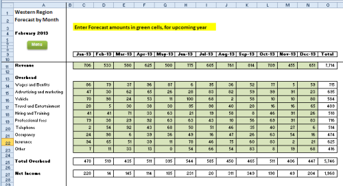
It has a traditional layout, with months across the columns, and budget categories down the side.

There are separate sheets for the Forecast amounts and the Actual amounts – and their layouts have to be exactly the same.

Here’s the Forecast sheet, where you enter the amounts in the green cells.

Time for an Update

In that sample file, I checked the file properties, and that workbook was created way back in September 2002! It was time for a new version of the budget workbook.

There’s a new download file now — #2 in the download section. This version takes a different approach for entering and reporting the budget amounts. Here’s what the new report looks like, and there are details below.

Named Table for Data Entry

Instead of entering the Forecast and Actual amounts horizontally, the new workbook has a named table for data entry – tblInput.

Enter the Forecast amounts there, and later, add the Actual amounts, when they’re available.

Calculated Budget Variance

The data entry table also has columns with formulas to calculate the Year to Date (YTD) amounts, and the Variance.

For YTD, the actual amount is used, if it has been entered. Otherwise, the forecast amount is used.

=IF([@Actual]=””,[@Forecast],[@Actual])

For Variance, the Forecast is subtracted from the Actual, or zero is shown, if there is no Actual amount.

=IF([@Actual]=””,0,[@Actual]-[@Forecast])

For Variance %, Actual is divided by Forecast, and 1 is subtracted, or zero is shown, if there is no Actual amount.

=IF([@Actual]=””,0,[@Actual]/[@Forecast]-1)

Report Types

On another sheet (Lists), there is a named table (tblRpt), with the five report types that will be available.

In the adjacent column, the number format for each report type is entered.

NOTE: The report types are an exact match for the columns in the data entry table.

There is also a pivot table based on the Report types table, with the Reports field in the Rows area.

The value in cell I2 will be used in a “Report” formula, to determine which values to show in our Budget report.
The pivot table name was changed to ptRptSel

Report Format

In a cell named FormatSel, a formula returns the format for the report type in cell I2

=INDEX(tblRpt[Format],MATCH(I2,tblRpt[Reports],0))

That value will be used in a macro that formats the final report.

Report Type Slicer

The next step is to insert a Slicer, based on the Report Type pivot table. This will be used to select which values to show in the final report.

Change the Slicer settings to hide the headings, and set it to show 5 columns

Adjust the Slicer’s size, so the five Report Types are visible. The Slicer will be moved to a different sheet later.

Report Value Calculation

Back on the Data Entry sheet, the final column in the input table is “Report” This column has a formula that gets the value based on the Report Type in cell I2 on the Lists sheet :

=INDEX(tblInput[@[Code]:[Var%]], MATCH(Lists!$I$2, tblInput[#Headers],0))

Currently, cell A2 show “Actual”, so that value is returned in the Report column.

Pivot Table Budget Report

To create the budget report, insert a pivot table, based on the input table.

Put the Category, Code and Item fields in the Row area, Month in the Column area, and Report in the Values area.
Change the pivot table name to ptRpt
Move the Slicer, so it is above the pivot table.

If you click a Report Type in the Slicer, and then refresh the pivot table, the values will change. We’ll be adding a macro, to automate that.

Macro to Update the Pivot Table

We’ll add a macro to update the pivot table’s Report values automatically, when we click a Report Type on the Slicer. The macro will also format the numbers, based on our lookup table.

To add the code:

Right-click the Lists sheet tab, and click View Code
Copy the following code, and paste it onto the code module

Private Sub Worksheet_PivotTableUpdate _
  (ByVal Target As PivotTable)
Dim pt As PivotTable

Select Case Target.Name
  Case "ptRptSel"
    Set pt = Sheets("Report") _
      .PivotTables("ptRpt")
    With pt
      .RefreshTable
      .PivotFields("Sum of Report") _
        .NumberFormat = Sheets("Lists") _
          .Range("FormatSel").Value
    End With
End Select
End Sub

Test the Report Type Slicer

After the macro has been added, go back to the Report sheet, and test the Slicer.

Click a report type in the Slicer, and see those values in the pivot table.
The Report column in the data entry table calculates which value to show
The macro refreshes the pivot table values, and applies the number format.

In the animated screen shot below, you can see that the blue text changes, when the Slicer is clicked. That cell is linked to cell I2 on the Lists sheet, to show the selected Report Type.

Another Budget Report Slicer

In the sample file, there’s another Slicer too — use it to show or hide the zeros on the Budget Report sheet.

That slicer is based on another named table and pivot table (ptZeros) on the Lists sheet.

There’s an extra section added to the code on the Lists sheet, to show or hide the zeros on the Budget Report sheet.

  Case "ptZeros"
    With ActiveWindow
      Select Case Range("ZeroSel").Value
        Case "Hide 0s"
          .DisplayZeros = False
        Case Else
          .DisplayZeros = True
      End Select
    End With

Get the Budget Report Workbook

To get the Budget Report with Value Selector workbook, go to the Budget Variance page on my website.

This example is #2 in the download section. The zipped file is in xlsm format, and contains macros.

__________________________