Someone sent me a workbook in which a simple VLOOKUP formula was returning #N/A errors, instead of the correct results. The product numbers looked the same, but Excel didn’t match them in the lookup. Can you solve this VLOOKUP formula error mystery?
VLOOKUP Formula Error
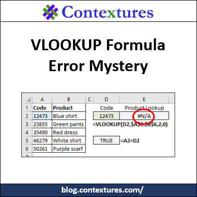
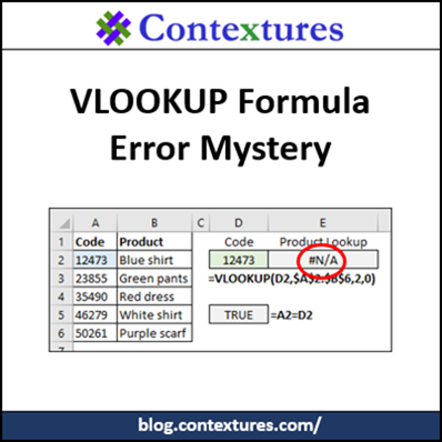
To show you the problem, here’s a screenshot of the lookup table, and the VLOOKUP formula. The formula in cell D5 says that the blue cell (A2) and the green cell (D2) are equal.
However, there’s a VLOOKUP formula error in cell E2. Instead of returning the product name, “Blue shirt”, the result is #N/A.

Get the VLOOKUP Sample File
If you love an Excel challenge, click here to download the sample file, and see if you can fix the problem – it’s a tricky one!
- If you’re not sure where to start looking for the problem, there are VLOOKUP troubleshooting tips on my site.
- The sample file also has a sheet that shows my troubleshooting steps, and another sheet shows my formula that fixes the problem.
WARNING – The troubleshooting steps for the VLOOKUP formula mystery start in the next section.
Stop reading here, if you don’t want to see how I fixed the VLOOKUP formula error.
.
.
.
.
.
VLOOKUP Troubleshooting Part 1
Usually, this type of VLOOKUP error occurs when one value is a real number, and the other is text number. See the details for that type of Number/Text problem on my website.
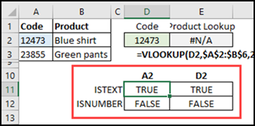
To test the numbers in the sample file, I used the ISTEXT and ISNUMBER functions. The screen show below shows the results of that test, for the values in A2 and D2.
Both cells contain text, not real numbers, so a Number/Text issue isn’t causing the errors in this workbook.
VLOOKUP Troubleshooting Part 2
Another common cause for VLOOKUP errors is extra characters in one of the cells – usually extra space characters.
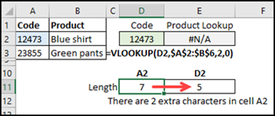
Using the LEN function, I checked the length of the string in each cell.
There are 7 characters in A2, and only 5 characters in cell D2
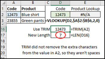
The TRIM function will remove leading, trailing, and duplicate spaces.
- In cell D16, I used TRIM on the value in A2.
- Then, I checked the length of the trimmed string.
There was no change, so the extra characters are NOT normal space characters.
VLOOKUP Troubleshooting Part 3
The next step is to figure out what those extra characters are.
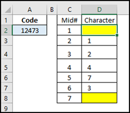
- We know there are 7 characters in cell A2, so I listed the numbers 1-7 on a worksheet.
- In the next column, the MID function extracts one character at each position.
The numbers from cell A2 appear in positions 2-6, and there are hidden characters at the start and end of the string.
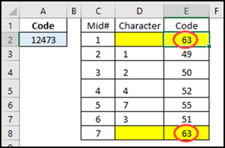
In the next column, I used the CODE function, to see what each character number is. Some characters, such as non-printing characters 0-30, can be removed with the CLEAN function. Let’s see if our hidden characters are one of those.
No, Excel says that cells D2 and D8 contain character #63.
There isn’t a non-printing character with code 63 though, so what is happening?
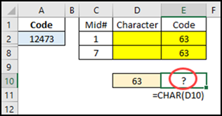
I typed 63 in cell D10, and used the CHAR function to see the character with that code number. Hmmm…it’s a question mark.
So those hidden characters are not really questions marks, but Excel is confused, and returns that code number anyway. (I found that clue on the Mr. Excel forum).
- CODE and CHAR use the basic ANSI character set in Windows, which has a maximum code number of 255.
- The hidden characters are probably from a different character set, and have a code number greater than 255
Whatever they are, we can’t use CLEAN to remove those hidden characters.
VLOOKUP Troubleshooting Part 4
To fix the formula, we don’t need to know what those hidden characters are. However, I was curious to find out if they were both the same character, or two different characters.
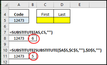
- To test that, I used SUBSTITUTE, to replace any instances of the first hidden character, with an empty string. That reduces the string by 1 character
- When I used SUBSTITUTE for each of the characters, both hidden characters were removed from the string.
If you really need to identify one of these strange characters, use the AscW function in a macro, or in the Immediate Window. This bit of code will show the character number for the first character in the active cell.
Sub GetCode()
  Debug.Print AscW(ActiveCell.Value)
End Sub
With that code, I learned that the hidden characters in this file are characters 8237 (cell C5) and 8236 (cell D5)
Solution to VLOOKUP Formula Error
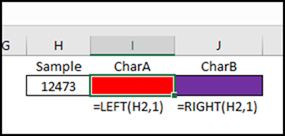
To fix the problem, I set up a “hidden character extraction range”.
- In cell H2, a sample code was pasted from the lookup table
- In cell I2, a LEFT formula pulls out the first character: =LEFT(H2,1)
- In cell J2, a RIGHT formula pulls out the last character: =RIGHT(H2,1)
NOTE: You could put this information on a hidden sheet. I left them on the same sheet as the VLOOKUP, so it’s easier to see how they’re used.
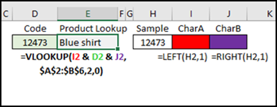
Then, combine those hidden characters with the product number in the VLOOKUP formula in cell E2, to get the product name:
=VLOOKUP(I2 & D2 & J2, $A$2:$B$6,2,0)
Get the Sample Workbook
To see all the details on the VLOOKUP Formula error problem and fix, download the sample file.
The zipped file is in xlsx format, and does not contain any macros.
More VLOOKUP Help
__________________________

Great! Literally, to a character, just dealt with a vlookup not working because UNICHAR(8236) and UNICHAR(8237) “hidden” in a cell.
Thank you.