
To make it easy for people to enter data on a worksheet, you can insert a check box control, using the Form Control tools on the Developer Tab. Then, use check box result in Excel formula solutions.
Form Controls on Developer Tab
If you don’t see a Developer tab, there are instructions here for showing it.

Adding these controls to a worksheet can make it easy for people to enter data – they just click to select the option that they want.

But, after they’ve checked that box, how do you capture that information, and use it in your formulas?
Link the Check Boxes to Cells
When you add a check box to the worksheet, it isn’t automatically linked to a cell. If you want to use the check box result in a formula, follow these steps to link it to a cell:
- To select a check box, press the Ctrl key, and click on the check box
- Click in the Formula Bar, and type an equal sign =
- Click on the cell that you want to link to, and press Enter

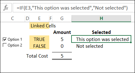
Check Box Result is TRUE or FALSE
If you have multiple check boxes, you can link each one to a separate cell on the worksheet.
In the screen shot below, Option 1 check box is linked to cell E3, and Option 2 is linked to cell E4. When the box is checked, the linked cell shows TRUE, and if it is not checked, the linked cell shows FALSE.

Use the Check Box Result in a Formula
In this example, each option has a price, and I’ve entered the prices in column B.

In a worksheet formula, if you use TRUE or FALSE in a calculation:
- TRUE has a value of 1.
- FALSE has a value of 0.
So, we can use the results in the linked cells, to calculate the cost for each option. We’ll multiply the cost in column B, by the check box result in column E.
- The formula in cell G3 is: =B3 * E3 and the result is 5, because 5 multiplied by 1 equals 5.
- In cell G4, the result is 0, because 10 multiplied by 0 equals 0.

Test the Result with IF
If your formula is fancier than a simple multiplication, you can use the IF function to test the result in the linked cell.
In cell H3, the following formula shows a text string if cell E3 is TRUE, and a different message if it is not TRUE.
=IF(E3,”This option was selected”,”Not selected”)

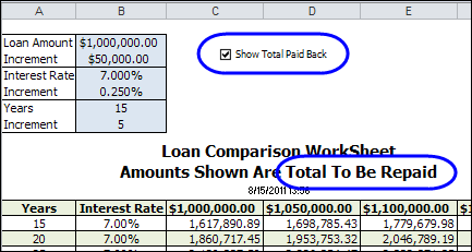
Another Check Box Formula Example
To see another example of using a check box result in a formula, take a look at Dave Peterson’s loan table formula on my Contextures website. There is a sample file that you can download.
A check box at the top of the worksheet is linked to cell C1. Check that box if you want to see the total amount that will be paid back, instead of the monthly payment required.
If cell C1 is TRUE, then the monthly payment in the table is multiplied by the number of payments. If C1 is FALSE, the monthly payment is multiplied by 1.
This is the formula in cell C12:
=-PMT($B12/12,12*$A12,C$11)*IF($C$1,$A12*12,1)
_____________________
Is it possible to insert a column and add enough checkboxes to match the rows of data needed? I can’t insert one checkbox at a time and readjust each box…
Thanks,
Jonathan
@Jonathan, there is code on my website for inserting check boxes into a range of cells
Using excel please design a formula to use a checkbox if checked then multiply by 7%
Hi Debra,
Great information. I have a spreadsheet where we track jobs and the collection of documents. I have 5 columns with check boxes that are checked as each document arrives back in the office. The order they arrive in can be random. I would like to use conditional formatting to colour rows once all the boxes are checked. I was also wondering if check boxes could be created as new jobs are added to the list or do I have to continually add spare rows of check boxes. We use about 500 rows per year and I can clear completed rows to start a new year but I am not sure how this affects associated check boxes. I currently have an automated sort/hide button that uses a macro to sort the rows and then filter the rows to only show jobs that are incomplete.
Hi Jeff,
Wow, that’s a lot of check boxes to manage on a worksheet! You’d have to keep adding them to new rows, throughout the year.
If you want to keep track of what’s filled in, those check boxes would need to be linked to cells in that row, so you could count the number of TRUE cells.
Could you get rid of the check boxes, and just have people put an X in the cell instead? Then you wouldn’t have to worry about links, and could just use a COUNTIF formula to count the number of Xs.
Thanks Debra, That is actually how I have been doing it and I guess we’ll go back to it. I just thought check boxes would be easier so I added them but it looks like it complicates things more than needed. Thanks for the insight. Great Blog by the way!
Hi. Good Day! :)) How can i make a responsive checkbox in MS Excel. Once i click the checkbox it will give 1 in respond and then after the process complete it will have the tally form below as total the checks i did? Thank you so much.. <3
Thank you for the solution. It helped me a lot.
I am working on a roster for a daycare. I have a list of the students and for each student I need 5 checkboxes for the days of the week (M-F). Based on the boxes checked, another sheet displays the time the child attends, i.e, if Monday=TRUE, display time, etc. I’m using VLOOKUP to get the times but need to populate only the day of the week cells that the child attends.
@Brian, in your IF formula, use 2 VLOOKUP functions.
–The first one would get the value for Monday
–The second one would get the time, if Monday is TRUE.
–If Monday is FALSE, the result is an empty string “”
For example,
=IF(VLOOKUP(A2,Sheet2!$A$2:$D$30,2,0)=TRUE,
VLOOKUP(A2,Sheet2!$A$2:$D$30,4,0),””)