

Use INDEX and MATCH together, for a powerful lookup formula. It’s similar to a VLOOKUP formula, but more flexible — the item that you’re looking for doesn’t have to be in the first column at the left. Watch the video to see how it works (there are written instructions too), and download the sample workbook to follow along.
Excel Lookup With Two Criteria
Watch this video to see how INDEX and MATCH work together — first with one criterion, and then with multiple criteria. Download the sample workbook to follow along, and the written instructions are below the video.
- 0:00 Introduction
- 0:26 Lookup with One Criterion
- 1:52 Test Each Criterion
- 2:22 Test With a Formula
- 3:26 Multiply the Results
- 4:03 INDEX / MATCH Formula
- 5:20 Check the Formula
- 5:57 Get the Sample File
Get Item Price with INDEX and MATCH
To see how INDEX and MATCH work together, we’ll start with an example that has only 1 criterion. Our price list has item names in column B, and we want to get the matching price from column C.
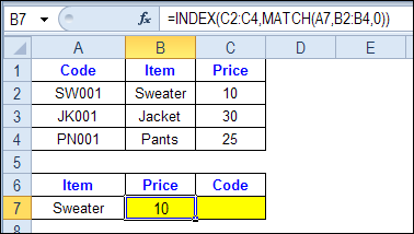
In the screen shot below, cell A7 has the name of the item that we need a price for – Sweater.
We can enter an INDEX and MATCH formula in cell C7, to get the price for that item:
=INDEX($C$2:$C$4,MATCH(A7,$B$2:$B$4,0))
How the INDEX and MATCH Formula Works
Here’s how the two functions work together:
- MATCH function gets the location of an item in a list
- INDEX function returns a value from a specific location in a list.
So, in our formula:
- the MATCH function looks for “Sweater” in the range B2:B4.
- The result is 1, because “Sweater” is item number 1, in that range of cells.
- the INDEX function looks in the range C2:C4
- The result is 10, from row 1 in that range
So, by combining INDEX and MATCH, you can find the row with “Sweater” and return the price from that row.
Find a Match for Multiple Criteria
In the first example, there was only one criterion, and the match was based on the Item name – Sweater. However, sometimes life, and Excel workbooks, are more complicated.
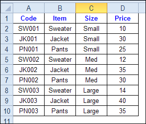
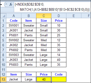
In the screen shot below, each item is listed 3 times in the pricing lookup table. We want to find the price for a large jacket.
To get the right price, you’ll need to use 2 criteria:
- the item name
- the size
Does it MATCH? True or False
Instead of a simple MATCH formula, we’ll use one that checks both the Item and Size columns.
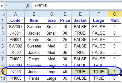
To see how this formula will work, I’ll temporarily add columns to check the item and Size of each item — is the item a Jacket, and is the Size a Large?
Enter this formula in E2, and copy down to E10: =C2=$C$13
Enter this formula in F2, and copy down to F10: =D2=$D$13
- If the Item in column B is a Jacket, the result in column E is TRUE. If not, the result is FALSE
- If the Size in column C is Large, the result in column F is TRUE. If not, the result is FALSE
To see if both results are TRUE in each row, enter this formula in G2, and copy down to G10: =F2*G2
When you multiply the TRUE/FALSE values,
- If either value is FALSE (0), the result is zero
- If both values are TRUE, the result is 1
Only the 8th row in our list of items has a 1, because both values are TRUE in that row.
We can tell the MATCH function to look for a 1, and that will return the information that we need.
Use MATCH With Multiple Criteria
Instead of adding extra columns to the worksheet, we can use an array-entered INDEX and MATCH formula to do all the work.
Here is the formula that we’ll use to get the correct price, and the explanation is below:
=INDEX($D$2:$D$10,
MATCH(1,(A13=$B$2:$B$10) * (B13=$C$2:$C$10),0))
NOTE: This is an array-entered formula, so press Ctrl + Shift + Enter, instead of just pressing the Enter key.
How the Formula Works
In this INDEX and MATCH example,
- prices are in cells D2:D10, so that is the range that the INDEX function will use
- the item name is in cell A13
- the size is in cell B13.
The formula checks for the selected items in $B$2:$B$10, and sizes in $C$2:$C$10. The results are multiplied.
- (A13=$B$2:$B$10)*(B13=$C$2:$C$10)
The MATCH function looks for the 1 in the array of results.
- MATCH(1,(A13=$B$2:$B$10)*(B13=$C$2:$C$10),0)
If you select that part of the formula and press the F9 key, you can see the calculated results. In the screen shot below there are 9 results, and all are zero, except the 8th result, which is 1.
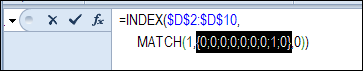
So, the INDEX function returns the price – 40 – from the 8th data row in column D (cell D9).
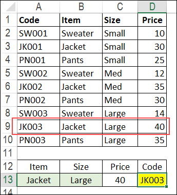
Get the Product Code
To find the product code for the selected item and size, you would change the formula to look in cells A2:A10, instead of the price column.
Put this formula in cell D13, and remember, this is an array-entered formula, so press Ctrl + Shift + Enter.
=INDEX($A$2:$A$10,
MATCH(1,(A13=$B$2:$B$10) * (B13=$C$2:$C$10),0))
In this example, the product code would be JK003, from cell A9.
Get the Workbook
To get the sample file with the Lookup Multiple Criteria examples, go to the Excel Lookup Multiple Criteria page on my Contextures site.
For more INDEX and MATCH tips and examples, visit the INDEX function and MATCH function page on the Contextures website. This is Example 4 in the sample file section of that page.
_____________
Hello,
I have tried to use the match index formula based on the above comments, bur getting error message NA.
=INDEX($O$5:$O$76,MATCH(1,(E8=$L$5:$L$76)*(E9=$M$5:$M$76),0))
Can someone let me know if am making any mistake in the above formula.
Shalini,
First of all, remember to use Ctrl + Shift + Enter when entering the formula.
That said, I believe #N/A message appears because there is no match for the criteria you select.
Make sure the combination you are trying to match really exists (E8 and E9).
I have the same problem, i need the #N/A to show as 0 instead. Please could someone help with this.
Thanks
AWESOME…..
I WAS STRUGGLING TO FIND SOLUTION TO EXTRACT DATA ON MULTIPLE CONDITIONS WITHOUT USING CONCATENATE FUNCTION… BUT WAS NT ABLE TO GET IT.
cONTEXTURES BLOG GAVE ME SOLUTION
THANKS A LOTTTTT……..
Hi!!! I’m trying to match all the available codes from an old coding version to a new one. For example, I got a Table with all the possible combination between codes. Also have another table that got service codes and its old codes, I need to match it with the table that got the possible combinations.
Example:
***CodeTable***
OldCode NewCode
013.2 A17.81
192.1 C70.0
192.1 C70.9
228.02 D18.02
346.7 G43.701
346.7 G43.711
346.7 G43.709
346.7 G43.719
784.51 R47.01
V12.54 Z86.73
***Service Codes***
ServiceCode OldCode NewCode
70450 013.2 ??????
70450 192.17 ??????
70450 228.02 ??????
70450 346.7 ??????
70450 784.51 ??????
70450 V12.54 ??????
I’ll appreciate your help…
My application has some blank spaces. Imagine in the example above if the first three items did not have code numbers. In other words, A2, A3 & A4 were blank. I am trying to achieve the rational that “code” only matters when there is a code, else ignore it. My formula is: =INDEX(Fb,MATCH(1,INDEX((A4=SYSTEM)*(B4=SPECIE)*(C4=SIZE)*(D4=GRADE),0),0))
For some systems, size isn’t pertinent and those cells are left blank. My formula works in all other combinations of system,specie,size, and grade but not when “size” is blank. I need to turn off the string *(C4=SIZE) when the cells in the “size” range are blank. In essence, I need to reduce the formula to: =INDEX(Fb,MATCH(1,INDEX((A4=SYSTEM)*(B4=SPECIE)*(D4=GRADE),0),0)) for certain values of “system”. Any ideas on how to do that?
Yeah, use an IF statement:
=IF(ISBLANK(SIZE), INDEX(Fb,MATCH(1,INDEX((A4=SYSTEM)*(B4=SPECIE)*(C4=SIZE)*(D4=GRADE),0),0)) , INDEX(Fb,MATCH(1,INDEX((A4=SYSTEM)*(B4=SPECIE)*(D4=GRADE),0),0)) )
Joaquim,
Thanks. I used =IF(OR(A4=”MSR”,A4=”MEL”),INDEX(Fb,MATCH(1,INDEX((A4=SYSTEM)*(B4=SPECIE)*(D4=GRADE),0),0)),INDEX(Fb,MATCH(1,INDEX((A4=SYSTEM)*(B4=SPECIE)*(C4=SIZE)*(D4=GRADE),0),0)))
We are thinking alike, but my new problem is that it only works as long as it is in the same worksheet as the ranges. I need index/match to work across workbooks. My data workbook “DESIGNVALUES” contains all of the design values. Each project workbook needs to retrieve design values from “DESIGNVALUES” but I haven’t been able to get index/match to work unless it is in the same worksheet with the data ranges. I have searched several blogs and it is a common topic but so far I’ve not seen a solution. People who say that it should work in 2010 haven’t tried it. I don’t know if it will work in 2013.
Dear all,
Good evening,
Anyone can help me to my problem, I have two working worksheet in excel
1. as my data entry, which you can find in every column the date, passport number, name, training course, result(Passed,Failed,No Show). I have more than a thousand person name with corresponding passport number and every person have more than twenty training need to attend. Mean in one person need to view a more line if your find it with a different date taken and result.
2. second worksheet have passport number and all training course title in horizontal line.
in the second worksheet under the training title the argument(condition) should be, if passport number(second worksheet) match to passport number(first worksheet), training course title(second worksheet match to training course column of the first worksheet, then check in the column of result(first worksheet) if found passed must to appear the date of was taken in the column of training course title in the second worksheet. what is the best formula for excel to get this. thanks