

Use INDEX and MATCH together, for a powerful lookup formula. It’s similar to a VLOOKUP formula, but more flexible — the item that you’re looking for doesn’t have to be in the first column at the left. Watch the video to see how it works (there are written instructions too), and download the sample workbook to follow along.
Excel Lookup With Two Criteria
Watch this video to see how INDEX and MATCH work together — first with one criterion, and then with multiple criteria. Download the sample workbook to follow along, and the written instructions are below the video.
- 0:00 Introduction
- 0:26 Lookup with One Criterion
- 1:52 Test Each Criterion
- 2:22 Test With a Formula
- 3:26 Multiply the Results
- 4:03 INDEX / MATCH Formula
- 5:20 Check the Formula
- 5:57 Get the Sample File
Get Item Price with INDEX and MATCH
To see how INDEX and MATCH work together, we’ll start with an example that has only 1 criterion. Our price list has item names in column B, and we want to get the matching price from column C.
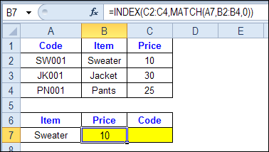
In the screen shot below, cell A7 has the name of the item that we need a price for – Sweater.
We can enter an INDEX and MATCH formula in cell C7, to get the price for that item:
=INDEX($C$2:$C$4,MATCH(A7,$B$2:$B$4,0))
How the INDEX and MATCH Formula Works
Here’s how the two functions work together:
- MATCH function gets the location of an item in a list
- INDEX function returns a value from a specific location in a list.
So, in our formula:
- the MATCH function looks for “Sweater” in the range B2:B4.
- The result is 1, because “Sweater” is item number 1, in that range of cells.
- the INDEX function looks in the range C2:C4
- The result is 10, from row 1 in that range
So, by combining INDEX and MATCH, you can find the row with “Sweater” and return the price from that row.
Find a Match for Multiple Criteria
In the first example, there was only one criterion, and the match was based on the Item name – Sweater. However, sometimes life, and Excel workbooks, are more complicated.
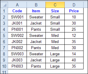
In the screen shot below, each item is listed 3 times in the pricing lookup table. We want to find the price for a large jacket.
To get the right price, you’ll need to use 2 criteria:
- the item name
- the size
Does it MATCH? True or False
Instead of a simple MATCH formula, we’ll use one that checks both the Item and Size columns.
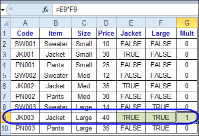
To see how this formula will work, I’ll temporarily add columns to check the item and Size of each item — is the item a Jacket, and is the Size a Large?
Enter this formula in E2, and copy down to E10: =C2=$C$13
Enter this formula in F2, and copy down to F10: =D2=$D$13
- If the Item in column B is a Jacket, the result in column E is TRUE. If not, the result is FALSE
- If the Size in column C is Large, the result in column F is TRUE. If not, the result is FALSE
To see if both results are TRUE in each row, enter this formula in G2, and copy down to G10: =F2*G2
When you multiply the TRUE/FALSE values,
- If either value is FALSE (0), the result is zero
- If both values are TRUE, the result is 1
Only the 8th row in our list of items has a 1, because both values are TRUE in that row.
We can tell the MATCH function to look for a 1, and that will return the information that we need.
Use MATCH With Multiple Criteria
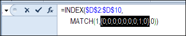
Instead of adding extra columns to the worksheet, we can use an array-entered INDEX and MATCH formula to do all the work.
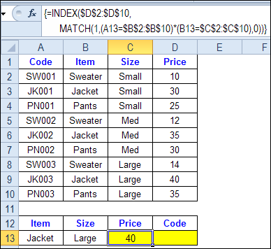
Here is the formula that we’ll use to get the correct price, and the explanation is below:
=INDEX($D$2:$D$10,
MATCH(1,(A13=$B$2:$B$10) * (B13=$C$2:$C$10),0))
NOTE: This is an array-entered formula, so press Ctrl + Shift + Enter, instead of just pressing the Enter key.
How the Formula Works
In this INDEX and MATCH example,
- prices are in cells D2:D10, so that is the range that the INDEX function will use
- the item name is in cell A13
- the size is in cell B13.
The formula checks for the selected items in $B$2:$B$10, and sizes in $C$2:$C$10. The results are multiplied.
- (A13=$B$2:$B$10)*(B13=$C$2:$C$10)
The MATCH function looks for the 1 in the array of results.
- MATCH(1,(A13=$B$2:$B$10)*(B13=$C$2:$C$10),0)
If you select that part of the formula and press the F9 key, you can see the calculated results. In the screen shot below there are 9 results, and all are zero, except the 8th result, which is 1.
So, the INDEX function returns the price – 40 – from the 8th data row in column D (cell D9).
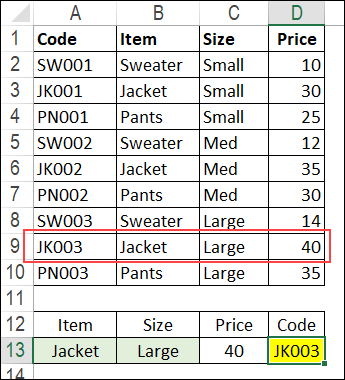
Get the Product Code
To find the product code for the selected item and size, you would change the formula to look in cells A2:A10, instead of the price column.
Put this formula in cell D13, and remember, this is an array-entered formula, so press Ctrl + Shift + Enter.
=INDEX($A$2:$A$10,
MATCH(1,(A13=$B$2:$B$10) * (B13=$C$2:$C$10),0))
In this example, the product code would be JK003, from cell A9.
Get the Workbook
To get the sample file with the Lookup Multiple Criteria examples, go to the Excel Lookup Multiple Criteria page on my Contextures site.
For more INDEX and MATCH tips and examples, visit the INDEX function and MATCH function page on the Contextures website. This is Example 4 in the sample file section of that page.
_____________
=IF(C12=”STD”,INDEX(EQ!$B$10:$K$11,MATCH(EQ!$B$52,EQ!$B$10:$B$11,0),MATCH(EQ!B13,EQ!$B$10:$K$10),IF(C12=”LED”,INDEX(‘EQ1’!$B$10:$K$11,MATCH(‘EQ1′!$B$52,’EQ1’!$B$10:$B$11,0),MATCH(‘EQ1′!B13,’EQ1’!$B$10:$K$10)))))
Hi, i hope you can help me.
i want to lookup data in 2 defferent =EQ= and =EQ1= worksheets by changing the data =MainPage= worksheet by changing data in cell c12 on =MainPage+
Sended on the 12 July but no response yet, can somebody please help
You did a few errors:
1) referring to a cell using ‘EQ1’!$B$10 instead of EQ1!$B$10
2) MATCH() has 3 arguments. If you don’t specify the third argument, MATCH will find the largest value that is less than or equal to lookup_value
3) you forgot some brackets. You need to put INDEX inside brackets.
4) you might want to specify the value_if_false argument in your second if. I would put something like “error” or “not found”.
You want =IF(C12=”STD”, INDEX() , IF(C12=”LED”, INDEX() , “not found” ) )
I was hoping someone could help me with my problem as follows;
Column A B C D E F G H I J
Concentrates Blend Mineral Concentrate Soya 21 10 11 11 10
And so on, I have more columns than this and lots of rows of date. What I would like to do in column K is total what is concentrates, ie 32, in column L total blend which is 10 and so on.
Please could someone advise a formula I can use. Thank you
Hi,
By using Index and Match formula how we can get Multiple result.
Example:
Row Labels Sum of Catches7
Dnyaneshwar Vaidya 2
Rohan Handibag 1
Farhan Nehari 2
Sandip Ghule 1
In given example Two Person Names Having same Value.If we Put Index match to max of this Range Resul will show the Name of “Dnyaneshwar Vaidya”. But same value is against another Person also.So How to get Both the Names or all the Name of Same Value if available.
Please help me in this.
Hi All,
I have data in sheet one with employee Id number, month and Hours Billed Data ranging from column C to P Now I want the data on sheet 2 where I want the Hours billed data for specific id(which repeats multiple times in column C2:C95) for specific month in column L2:L95 the result the match for C and L Hours billed in sheet2? Anyone can help
How to select value for A-152-4 as 33 and B-152-4 as 304 using multiple index & match formula . Pl help me
1 2 3 4 5 6 7 8 9 10 11
A
147 201 202 203 204 205 206 207 208 209 210 211
152 30 31 32 33 34 35 36 37 38 39 40
136 50 51 52 53 54 55 56 57 58 59 60
852 70 71 72 73 74 75 76 77 78 79 80
963 90 91 92 93 94 95 96 97 98 99 100
B
147 101 102 103 104 105 106 107 108 109 110 111
152 301 302 303 304 305 306 307 308 309 310 311
136 501 502 503 504 505 506 507 508 509 510 511
852 701 702 703 704 705 706 707 708 709 710 711
963 901 902 903 904 905 906 907 908 909 910 911
sir we have one problem plz solve this
,=INDEX(performance!$E$2:$L$301,MATCH(today!$E2&today!$F2&today!$G2&today!$H2&today!$I2&today!$J2&today!$K2,performance!$E$2:$E$301&performance!$F$2:$F$301&performance!$G$2:$G$301&performance!$H$2:$H$301&performance!$I$2:$I$301&performance!$J$2:$J$301&performance!$K$2:$K$301,0),8)
this formula was given exject but we want +/- 3% range between plz solve my problem
thank u Advance