

Use INDEX and MATCH together, for a powerful lookup formula. It’s similar to a VLOOKUP formula, but more flexible — the item that you’re looking for doesn’t have to be in the first column at the left. Watch the video to see how it works (there are written instructions too), and download the sample workbook to follow along.
Excel Lookup With Two Criteria
Watch this video to see how INDEX and MATCH work together — first with one criterion, and then with multiple criteria. Download the sample workbook to follow along, and the written instructions are below the video.
- 0:00 Introduction
- 0:26 Lookup with One Criterion
- 1:52 Test Each Criterion
- 2:22 Test With a Formula
- 3:26 Multiply the Results
- 4:03 INDEX / MATCH Formula
- 5:20 Check the Formula
- 5:57 Get the Sample File
Get Item Price with INDEX and MATCH
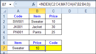
To see how INDEX and MATCH work together, we’ll start with an example that has only 1 criterion. Our price list has item names in column B, and we want to get the matching price from column C.
In the screen shot below, cell A7 has the name of the item that we need a price for – Sweater.
We can enter an INDEX and MATCH formula in cell C7, to get the price for that item:
=INDEX($C$2:$C$4,MATCH(A7,$B$2:$B$4,0))
How the INDEX and MATCH Formula Works
Here’s how the two functions work together:
- MATCH function gets the location of an item in a list
- INDEX function returns a value from a specific location in a list.
So, in our formula:
- the MATCH function looks for “Sweater” in the range B2:B4.
- The result is 1, because “Sweater” is item number 1, in that range of cells.
- the INDEX function looks in the range C2:C4
- The result is 10, from row 1 in that range
So, by combining INDEX and MATCH, you can find the row with “Sweater” and return the price from that row.
Find a Match for Multiple Criteria
In the first example, there was only one criterion, and the match was based on the Item name – Sweater. However, sometimes life, and Excel workbooks, are more complicated.
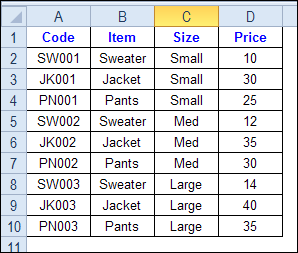
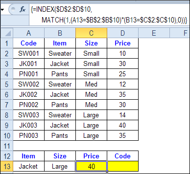
In the screen shot below, each item is listed 3 times in the pricing lookup table. We want to find the price for a large jacket.
To get the right price, you’ll need to use 2 criteria:
- the item name
- the size
Does it MATCH? True or False
Instead of a simple MATCH formula, we’ll use one that checks both the Item and Size columns.
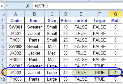
To see how this formula will work, I’ll temporarily add columns to check the item and Size of each item — is the item a Jacket, and is the Size a Large?
Enter this formula in E2, and copy down to E10: =C2=$C$13
Enter this formula in F2, and copy down to F10: =D2=$D$13
- If the Item in column B is a Jacket, the result in column E is TRUE. If not, the result is FALSE
- If the Size in column C is Large, the result in column F is TRUE. If not, the result is FALSE
To see if both results are TRUE in each row, enter this formula in G2, and copy down to G10: =F2*G2
When you multiply the TRUE/FALSE values,
- If either value is FALSE (0), the result is zero
- If both values are TRUE, the result is 1
Only the 8th row in our list of items has a 1, because both values are TRUE in that row.
We can tell the MATCH function to look for a 1, and that will return the information that we need.
Use MATCH With Multiple Criteria
Instead of adding extra columns to the worksheet, we can use an array-entered INDEX and MATCH formula to do all the work.
Here is the formula that we’ll use to get the correct price, and the explanation is below:
=INDEX($D$2:$D$10,
MATCH(1,(A13=$B$2:$B$10) * (B13=$C$2:$C$10),0))
NOTE: This is an array-entered formula, so press Ctrl + Shift + Enter, instead of just pressing the Enter key.
How the Formula Works
In this INDEX and MATCH example,
- prices are in cells D2:D10, so that is the range that the INDEX function will use
- the item name is in cell A13
- the size is in cell B13.
The formula checks for the selected items in $B$2:$B$10, and sizes in $C$2:$C$10. The results are multiplied.
- (A13=$B$2:$B$10)*(B13=$C$2:$C$10)
The MATCH function looks for the 1 in the array of results.
- MATCH(1,(A13=$B$2:$B$10)*(B13=$C$2:$C$10),0)
If you select that part of the formula and press the F9 key, you can see the calculated results. In the screen shot below there are 9 results, and all are zero, except the 8th result, which is 1.
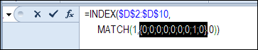
So, the INDEX function returns the price – 40 – from the 8th data row in column D (cell D9).
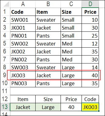
Get the Product Code
To find the product code for the selected item and size, you would change the formula to look in cells A2:A10, instead of the price column.
Put this formula in cell D13, and remember, this is an array-entered formula, so press Ctrl + Shift + Enter.
=INDEX($A$2:$A$10,
MATCH(1,(A13=$B$2:$B$10) * (B13=$C$2:$C$10),0))
In this example, the product code would be JK003, from cell A9.
Get the Workbook
To get the sample file with the Lookup Multiple Criteria examples, go to the Excel Lookup Multiple Criteria page on my Contextures site.
For more INDEX and MATCH tips and examples, visit the INDEX function and MATCH function page on the Contextures website. This is Example 4 in the sample file section of that page.
_____________
Hi,
SIR I HAVE A SHEET IN WHICH I HAVE 6 COLUMNS FOR RICE INVENTORY.
1)Report No
2)IN/OUT/PROCESS/Fg(This column show whether Rice In, out,Proceeds & Finshed goods)
3)Product Name
4) In (If In & FG i have make entry of quantity in this column)
5) Out (If out or process i have make entry of quanitity in this column)
6) Balance
Now i want that balance column check the report number, product name , & whether it is IN OUT Or other so it give me balance
If it is IN or FG so it add or if it out or Process its less it.
Hai,
Please tell me how I can retrieve data from below two worksheets
sheet 1:
Date Sales
15/10/2013 Honda
20/10/2013 Benz
23/10/2013 Toyota
Sheet 2:
Date Sales
if I enter the date on the second sheet, how I can retrieve sales data using formula
Hoping to hearing from you soon
Thanks
=IF(C12=”STD”,INDEX(EQ!$B$10:$K$11,MATCH(EQ!$B$52,EQ!$B$10:$B$11,0),MATCH(EQ!B13,EQ!$B$10:$K$10),IF(C12=”LED”,INDEX(‘EQ1’!$B$10:$K$11,MATCH(‘EQ1′!$B$52,’EQ1’!$B$10:$B$11,0),MATCH(‘EQ1′!B13,’EQ1’!$B$10:$K$10)))))
Hi, i hope you can help me.
i want to lookup data in 2 defferent =EQ= and =EQ1= worksheets by changing the data =MainPage= worksheet by changing data in cell c12 on =MainPage+
Hi,
First of all, thanks for this article.
I have data like this..
Region State Segment Sales
Central Illinois Corporate 5.9
West Washington Corporate 13.01
West California Home Office 6362.85
East Massachusetts Home Office 232.95
Central Minnesota Small Business 1164.45
East New Hampshire Home Office 705.47
West Washington Consumer 299.74
like this, i have data more than 9000 rows for these 4 regions in random order.
I would like to see the data separately for regions. i.e all the rows of Central region should come as one data set and all the rows of East region should come as another data set and so on..
I did this using VLOOKUP function.
But i need the solution using INDEX and MATCH functions.
Please suggest me..
I don’t think I fully understand what you mean but it sounds like a problem you could solve using a pivot table
All of these tips are so very helpful for potenetial issues. I have not been able o identify how to pull my challenge into any of these formulas. Can anyone assist?
Columns/Row: C7 through H7 Display “Year 1” “Year 2” etc. through “Year 6”
Columns/Row: C30 through H7 Display a cumulaative total based on formulas in preceeding rows.
The goal is to return the year (in cell H33) when the “Positive Payback” has been achieved.
Example: C30 may be -365 / D30 may be -290 / E30 may be -188 / F30 may be 25 / G30 may be 150 / H30 may be 250
The end result should display “Year 4” Since this is the year it bacame a positive number.
Any ideas?
I have a trial balance from work which has account numbers vertically and company codes horizontally, along with account balances (data tab). I am trying to write a formula on another tab in the same workbook that will display the account balance based upon a specific company code and account number specified on another tab in the workbook. I have tried the index/match formula but cannot seem to get it to work. I am hoping to be able to replicate the formula, as well as drop new data (same format) into the data tab each month.
Any ideas?