

Use INDEX and MATCH together, for a powerful lookup formula. It’s similar to a VLOOKUP formula, but more flexible — the item that you’re looking for doesn’t have to be in the first column at the left. Watch the video to see how it works (there are written instructions too), and download the sample workbook to follow along.
Excel Lookup With Two Criteria
Watch this video to see how INDEX and MATCH work together — first with one criterion, and then with multiple criteria. Download the sample workbook to follow along, and the written instructions are below the video.
- 0:00 Introduction
- 0:26 Lookup with One Criterion
- 1:52 Test Each Criterion
- 2:22 Test With a Formula
- 3:26 Multiply the Results
- 4:03 INDEX / MATCH Formula
- 5:20 Check the Formula
- 5:57 Get the Sample File
Get Item Price with INDEX and MATCH
To see how INDEX and MATCH work together, we’ll start with an example that has only 1 criterion. Our price list has item names in column B, and we want to get the matching price from column C.
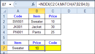
In the screen shot below, cell A7 has the name of the item that we need a price for – Sweater.
We can enter an INDEX and MATCH formula in cell C7, to get the price for that item:
=INDEX($C$2:$C$4,MATCH(A7,$B$2:$B$4,0))
How the INDEX and MATCH Formula Works
Here’s how the two functions work together:
- MATCH function gets the location of an item in a list
- INDEX function returns a value from a specific location in a list.
So, in our formula:
- the MATCH function looks for “Sweater” in the range B2:B4.
- The result is 1, because “Sweater” is item number 1, in that range of cells.
- the INDEX function looks in the range C2:C4
- The result is 10, from row 1 in that range
So, by combining INDEX and MATCH, you can find the row with “Sweater” and return the price from that row.
Find a Match for Multiple Criteria
In the first example, there was only one criterion, and the match was based on the Item name – Sweater. However, sometimes life, and Excel workbooks, are more complicated.
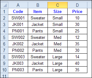
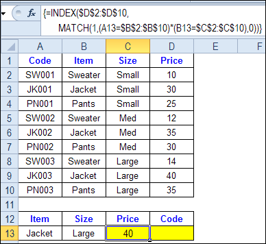
In the screen shot below, each item is listed 3 times in the pricing lookup table. We want to find the price for a large jacket.
To get the right price, you’ll need to use 2 criteria:
- the item name
- the size
Does it MATCH? True or False
Instead of a simple MATCH formula, we’ll use one that checks both the Item and Size columns.
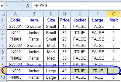
To see how this formula will work, I’ll temporarily add columns to check the item and Size of each item — is the item a Jacket, and is the Size a Large?
Enter this formula in E2, and copy down to E10: =C2=$C$13
Enter this formula in F2, and copy down to F10: =D2=$D$13
- If the Item in column B is a Jacket, the result in column E is TRUE. If not, the result is FALSE
- If the Size in column C is Large, the result in column F is TRUE. If not, the result is FALSE
To see if both results are TRUE in each row, enter this formula in G2, and copy down to G10: =F2*G2
When you multiply the TRUE/FALSE values,
- If either value is FALSE (0), the result is zero
- If both values are TRUE, the result is 1
Only the 8th row in our list of items has a 1, because both values are TRUE in that row.
We can tell the MATCH function to look for a 1, and that will return the information that we need.
Use MATCH With Multiple Criteria
Instead of adding extra columns to the worksheet, we can use an array-entered INDEX and MATCH formula to do all the work.
Here is the formula that we’ll use to get the correct price, and the explanation is below:
=INDEX($D$2:$D$10,
MATCH(1,(A13=$B$2:$B$10) * (B13=$C$2:$C$10),0))
NOTE: This is an array-entered formula, so press Ctrl + Shift + Enter, instead of just pressing the Enter key.
How the Formula Works
In this INDEX and MATCH example,
- prices are in cells D2:D10, so that is the range that the INDEX function will use
- the item name is in cell A13
- the size is in cell B13.
The formula checks for the selected items in $B$2:$B$10, and sizes in $C$2:$C$10. The results are multiplied.
- (A13=$B$2:$B$10)*(B13=$C$2:$C$10)
The MATCH function looks for the 1 in the array of results.
- MATCH(1,(A13=$B$2:$B$10)*(B13=$C$2:$C$10),0)
If you select that part of the formula and press the F9 key, you can see the calculated results. In the screen shot below there are 9 results, and all are zero, except the 8th result, which is 1.
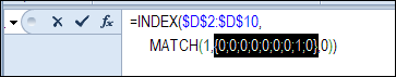
So, the INDEX function returns the price – 40 – from the 8th data row in column D (cell D9).
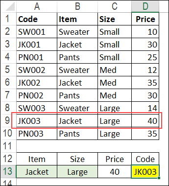
Get the Product Code
To find the product code for the selected item and size, you would change the formula to look in cells A2:A10, instead of the price column.
Put this formula in cell D13, and remember, this is an array-entered formula, so press Ctrl + Shift + Enter.
=INDEX($A$2:$A$10,
MATCH(1,(A13=$B$2:$B$10) * (B13=$C$2:$C$10),0))
In this example, the product code would be JK003, from cell A9.
Get the Workbook
To get the sample file with the Lookup Multiple Criteria examples, go to the Excel Lookup Multiple Criteria page on my Contextures site.
For more INDEX and MATCH tips and examples, visit the INDEX function and MATCH function page on the Contextures website. This is Example 4 in the sample file section of that page.
_____________
I am trying to use and Index & Match function where the matches are coming from a Data Validation List and the indexing criteria & matches are in another tab. It appears to me I’ve written the formula ok, but am still getting the #N/A result, which I’m guessing is because of the data validation list. Any thoughts? Below is the formula I’ve written.
{=INDEX(‘All Data’!$K:$K,MATCH($C$19&$E$19&$H$19,’All Data’!$A:$A&’All Data’!$C:$C&’All Data’!$E:$E,0),1)}
E19 & H19 are the match criteria from the data validation list. All three criteria need to be met in order to return the correct value in All Data column K.
I appreciate any help you can give me.
Hi. I am trying to compare two array and find duplicates, I already check for index, match do not work, and(exact do not work, conditional formatting countif do not work, let me give you a little example.
13 16 17 40 42 44 10 11 12 17 28 46
1 12 22 44 46 52 3 9 11 21 24 49
10 13 35 36 46 42 11 24 36 45 46 47
9 26 34 40 42 49 3 6 36 46 48 52
1 2 25 43 48 53 2 7 11 15 43 45
8 32 35 46 47 52 3 6 16 30 31 40
20 44 46 48 52 53 20 44 46 48 52 53
15 17 22 40 41 45 29 33 46 48 49 53
@victor you can use SUM and COUNTIF in an array-entered formula.
For example, if the first sets of numbers are in B2:G2, and I2:N2, put this formula in cell P2:
=SUM(COUNTIF(B2:G2,I2:N2))
Then, instead of pressing Enter, press Ctrl + Shift + Enter to array-enter the formula.
Copy the formula down to row 7.
sorry is two arrays 6by6 the first six are 13.16.17.40.42.44 compare against 10.11.12.17.28.46 and so on thanks.
Hi Debra, I tried but do not work.
@Vicktor what happened when you tried it?
What separator do you use in other formulas? Perhaps you need to use a semi-colon, instead of a comma:
=SUM(COUNTIF(B2:G2;I2:N2))
Thanks for your time, I write exactly what you say, but pop a message formula have error.
Did you press ctrl + shift + enter
Which separator did you use — comma or semi-colon?
the formula you type have an error, pop the same messages. thanks. anyway I got a vba code that resolve my problem.
again thank you so much for reading my post and tried to help. keep in touch.