Do you sometimes need to fix numbers with trailing minus signs, after you import data into Excel? I don’t run into this problem too often, but I usually fix them with the Text to Columns feature.
Text To Columns
Here’s how I fix the numbers in Text To Columns:
- Select the column that contains the trailing minus signs
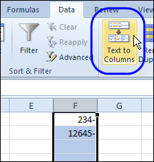
- On the Excel Ribbon’s Data tab, click Text to Columns.

- Click the Next button in Steps 1 and 2.
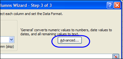
- In Step 3, click the Advanced button.

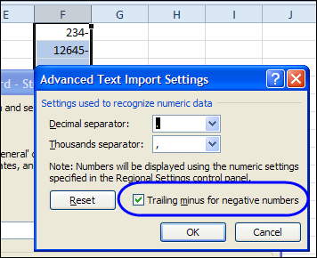
- Add a check mark to the option, “Trailing Minus for Negative Numbers”

- Click OK, and then click Finish.
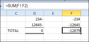
The minus signs are magically moved to the front of the numbers, and they’ll calculate correctly if you include them in formulas.

Fix Trailing Minus Signs With a Formula
If you need to fix trailing minus signs frequently, you might prefer a formula solution. With a formula, the numbers are fixed without your manual intervention, as soon as the data is pasted into the worksheet.
Thanks to Bob Ryan, from Simply Learning Excel, who sent this formula to fix imported numbers with trailing minus signs.
- In this example, the first number with a trailing minus sign is in cell A1
- Select cell B1, and enter this formula:
- =IF(RIGHT(A1,1)=”-“,-VALUE(LEFT(A1,LEN(A1)-1)),VALUE(A1))
- Copy the formula down to the last row of data.
In the formula, the RIGHT function returns the last character in cell A1.
If that character is a minus sign, the VALUE function returns the number value to the left of the trailing minus sign.
The minus sign before the VALUE function changes the value to a negative amount.
How Do You Fix Trailing Minus Signs?
Do you use another solution for trailing minus signs? There is a Trailing Minus Signs macro on the Contextures website, if you want to automate the fix.

@Hans,
Nice formula! A couple of points about it, though. Both our formulas report a wrong result for an entry like ‘2-4 (note the leading apostrophe)… my formula treats it as a serial date number (because the number on either side of the dash are small enough to be interpretted in my US system as month-day) where as your formula simply moves the dash to the front of the number returning -24 for its result. Your formula has an interesting anomoly built around the ‘2-4 type entry though. If your formula is already on the worksheet, change A1 to ‘2-4 and your formula returns -24 as discussed above; HOWEVER, if the value ‘2-4 is in A1 before your formula is placed on the worksheet, then when you enter your formula into a cell, it returns a series of # signs.
Rick Rohtstein
You have got a point there.
I never considered such subtleties as I have only (sometimes) used the formula after importing data from SAP where the only problem is the trailing minus signs.
If any of the methods explained on this webpage do not work, note that there are different “minus sign” characters, such as “‐” or “-” or “–” or “—”
I had been generating reports from a particular source which does not use the standard “-“, and this problem had plagued me for days before I mustered the determination to find the cause. You can imagine the feeling of satisfaction upon discovering the imposter “minus sign”.