
When you were first learning how to use Excel, you quickly discovered the basic Excel functions, like SUM, COUNT, MIN, MAX, and AVERAGE. Now you’re ready for advanced calculations, like how to find MIN IF or MAX IF in Excel.
Beyond the Basics with MIN IF
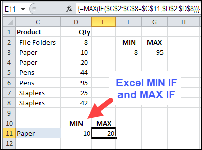
In this example, we want to see the MIN and MAX for a specific product. There is a SUMIF function and a COUNTIF function, but no MINIF or MAXIF.
- [Update]: In Excel 2019, and Excel for Office 365, you can use the new MINIFS and MAXIFS functions. There is more information on the MIN and MAX page on my Contextures site.
So, we’ll have to create our own MINIF formula, using MIN and IF. I’ve selected a product in cell C11, and the formula will be built in cell D11.
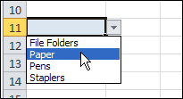
To make it easy to select a product, I created a drop down list of product names, by using data validation.
NOTE: You can also calculate MIN IF and MAX IF with Multiple Criteria
MIN IF Formula
The formula starts with the MIN and IF functions, and their opening brackets:
=MIN(IF(
Next, we want to find the rows where the product name matches the product in C11:
- Select C2:C8, where the product names are listed
- Type an = sign
- Click on cell C11
=MIN(IF(C2:C8=C11

Next, select D2:D8, where the quantities are listed. If the product name matches, we want to check the product quantity
=MIN(IF(C2:C8=C11,D2:D8

To finish the formula:
- Type two closing brackets
- Then press Ctrl+Shift+Enter to array-enter the formula.
=MIN(IF(C2:C8=C11,D2:D8))

NOTE: If you plan to copy this formula down a column, use absolute references to the product and quantity ranges:
=MIN(IF($C$2:$C$8=C11,$D$2:$D$8))
Array Entered Formula
If you select cell D11, and look at the formula in the Formula Bar, there are curly brackets at the start and end of the formula. Those were automatically added, because the formula was array-entered (Ctrl + Shift + Enter).
If you don’t see those curly brackets, you pressed Enter, instead of Ctrl + Shift + Enter.
To fix the formula:
- Click in the formula bar (it doesn’t matter where you click within the formula)
- Press Ctrl + Shift + Enter.

Create a MAXIF Formula
To find the maximum quantity for a specific product, use MAX instead of MIN.
=MAX(IF(C2:C8=C11,D2:D8))
or use absolute references for the product and quantity ranges:
=MAX(IF($C$2:$C$8=C11,$D$2:$D$8))
And remember to press Ctrl+Shift+Enter

Multiple Criteria for MIN IF or MAX IF
These formulas have only one criterion — the product name. If you’re ready for the next challenge, you can also calculate MIN IF and MAX IF with Multiple Criteria
- [Update]: In Excel 2019, and Excel 365, you can use the new MINIFS and MAXIFS functions. For more information, go to the MIN and MAX page on my Contextures site.
Watch the MIN IF or MAX IF Video
To see the steps for creating MIN IF and MAX IF formulas, watch this short Excel video tutorial. The sample file for this video can be downloaded from my Contextures website, on the MIN and MAX page.
________________________

________________
Great example! Thanks a lot!
Hi,thank you very much. I was able to do the same with LARGE function. The trick was to use Ctrl+Shift+Enter to array array-enter the formula and it worked as expected. Very kind of you to share this knowledge with us.
I’m having difficulties with the results as I have in my list dates instead of numbers, as you know dates are numbers as well. Also I have my list of variables ea A,B, C, D etc in which for A I have fro example 4 different dates and for B could be 2 different dates and C just one date and D could be 2 or 3 dates, now when applying the formula it brings for eac case the max date from the whole list not from the specific variable, can anybody help with this?
Hello Debra,
I am trying to return min and max dates but I keep getting 1/0/1900 as my date which is not accurate. Do you know what might be causing this?
Hi,
I have a file with a sheet (“Donations”) containing a list of donations. Each donor is tagged with an alphanumeric UID ending in letters which correspond to various criteria – an A in their UID means they’re an Active Member, X for ex-trustees, P for prospect donors, V for volunteers; a UID can have multiple letters if they meet more than one of those criteria.
Column B of my Sheet1 lists each of the unique criteria codes (P, V, X….). On the Donations sheet column A lists the UIDs and column D lists the donation given by each donor.
I can easily work out the total and average donation amounts for each of those criteria codes (where I’m looking up the criteria code in row 34):
=SUMIF(donations!A:A,”*”&B34&”*”,donations!D:D)
and
=AVERAGEIF(donations!A:A,”*”&B34&”*”,donations!D:D)
But how do I work out the minimum and maximum amounts given by each code? I’ve tried:
{=MIN(IF((donations!A:A=”*”&B34&”*”),(donations!D:D)))}
but it just gives me a zero value. I use Ctrl+Shift+Enter since it’s an array formula.
Can you help?
Love your work by the way.
Thanks!
You can use the SEARCH function to check for the letters, and ISNUMBER to test if a number was returned.
This is an array formula, so press Ctrl+Shift+Enter
=MIN(IF(ISNUMBER(SEARCH($B34,Donations!$A$2:$A$6)),Donations!$D$2:$D$6))
Same thing for MAX
=MAX(IF(ISNUMBER(SEARCH($B34,Donations!$A$2:$A$6)),Donations!$D$2:$D$6))
hi, i dont know why, but even if i copy the formula from this page, click ctl shift and enter it doest give me values, excel locks me asking if i am not trying to type formula.
and it show the pop up, just after i put ” ,” after =min(if(A1:A5;A7, please help
Depending on your regional settings, you might need to use a semi-colon as a separator, instead of a comma
=MIN(IF(A1:A5;A7;