
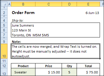
You’ve most likely heard this warning — “Avoid merged cells in your Excel worksheets!”, and that is excellent advice. Merged cells can cause problems, especially when they’re in a table that you’ll be sorting and filtering. You’ll run into more problems if you try to autofit merged cell row height.
Author: Debra Dalgleish
Compare Top and Bottom Sales in Pivot Table
An Excel pivot table is a great way to summarize a large amount of data, and with its Top 10 filter, you can compare the top values to the bottom values.
But don’t limit yourself to the Top 10 versus the Bottom 10 – dig deeper by using the other options in the filter.
Summarize the Data
With a few mouse clicks, you can summarize thousands of rows of data into a concise and informative pivot table.
In this example, there is a list of product, and their total sales over two years.

Sort by Sales Values
Instead of viewing the products alphabetically, you can sort by total sales, in descending order, to see the best selling products at the top of the list.
Here is the same list, with Oatmeal Raisin at the top.

Spotlight the Best Selling Products
Instead of showing all the products, you can use the pivot table’s Top 10 filter in the Product field, to filter the results.

The Top 10 filter is customizable, and can be used to show the top 3 items, instead of the top 10.

Top 3 Sales in Pivot Table
Here is the pivot table, with the Top 3 items showing, and the grand total for those items.

Compare to Bottom Items
If you’re working on a sales plan, you might want to decide where to focus your efforts, and a pivot table, or two, could help.
- If the top 3 products have total sales of approximately $136K, how are the bottom selling products doing, in comparison?
- How many of those bottom selling products are required to match the top 3 sales?
To find out, you can make a copy of the pivot table, and change the Top 10 filter. Instead of Top 3 Items, filter for Bottom Sum, and use the $136K amount as the target SUM.

Difference in Comparison Results
In this example, the top 3 sales were $136,165, and the bottom 10 products have sales of $173,489. The totals are not an exact match, because the pivot table filters for the products that total the specified sum, or more.

Find Best Results
The bottom 9 products don’t reach the target amount, so the 10th lowest product is also included. That puts the total over the target, and it shows that the best results come from a small number of products.
Focus your sales efforts there, and you might have a great sales year.

Watch the Pivot Table Top 10 Compare Video
To see the steps for comparing top and bottom values in a pivot table, you can watch this short Excel video tutorial.
________________
Trouble Counting Excel AutoFilters on Sheet
It seemed simple enough, but counting the AutoFilters on an Excel sheet is a tough job!
The answer to “How many worksheet AutoFilters are there?” is “It depends!”
You can read the fascinating (to me!) results below.
The Good Old Days
In the old days, before Excel 2003, you could only have one AutoFilter on a sheet. That’s pretty easy to count – either 1 or 0.
For example, this Excel 2010 sheet has a single list that is not a named table. An AutoFilter was applied to this list, and the AutoFilter arrows have been turned off.
If you point to one of the headings, where the hidden arrow is, the tooltip for that filter appears, so that shows us the AutoFilter is still active.

Count the Worksheet AutoFilters
To count the worksheet AutoFilters, I usually use AutoFilterMode to check if one exists.
Recently, Pascal (forum name: p45cal) emailed me, to suggest that checking for a worksheet AutoFilter would be more reliable. Thanks, Pascal, for inspiring this test!
Macro Code Count AutoFilters
This code tests for a worksheet AutoFilter, by using either AutoFilterMode or AutoFilter:
Sub CountSheetAutoFilters()
Dim iARM As Long
Dim iAR As Long
'counts all worksheet autofilters
'even if all arrows are hidden
If ActiveSheet.AutoFilterMode = True Then iARM = 1
    Debug.Print "AutoFilterMode: " & iARM
If Not ActiveSheet.AutoFilter Is Nothing Then iAR = 1
    Debug.Print "AutoFilter: " & iAR
End Sub
When I test that code in the Immediate window, both counting methods show 1 AutoFilter.

Named Table on the Worksheet
What happens if there is a named table on the worksheet, and it has its own AutoFilter? I ran the code again, on the worksheet shown below.
The worksheet has a named table, and it has an AutoFilter applied, with all the arrows hidden.

When I test the code in the Immediate window, both counting methods show zero AutoFilters.
I consider that count correct, because there is a ListObject with an AutoFilter, but no worksheet AutoFilter.

Different Count Results
In the screen shot above, you can see that cell A1 is selected – outside of the named table. When I selected cell B1, inside the table, and ran the code, the results were different. AutoFilterMode was still zero, but AutoFilter detected one.
Apparently, Excel is counting the active cell’s table as a worksheet AutoFilter, with the AutoFilter counting method. I’d rather go with the AutoFilterMode’s zero, and count the ListObject AutoFilters separately.

Test With Visible AutoFilter Arrows
Maybe the hidden arrows are affecting the results. To check, I ran code to show all the list AutoFilter arrows, and tested again.
The results were the same as in the previous tests, so visible arrows don’t make a difference.
Multiple Tables on Worksheet
For some final tests, I created a sheet with 3 lists:
- Named Table – no AutoFilter – no arrows
- Named Table – AutoFilter – visible arrows
- Worksheet table – AutoFilter – visible arrows
With a cell in Named Table 1 selected, AutoFilterMode counted one, and AutoFilter counted zero.
As in the previous test, the AutoFilter counting method is based on the active cell’s table AutoFilter. It doesn’t detect the AutoFilter in Worksheet Table 3.

And More Results
With any other cell in the worksheet selected, the results were different – both AutoFilter and AutoFilterMode counted one – the correct count of worksheet AutoFilters.

Counting Worksheet AutoFilters Conclusion
Because ActiveSheet.AutoFilter detects the AutoFilter in the active cell, it could cause a miscount of worksheet AutoFilters.
I’ll stick to the AutoFilterMode for a count of worksheet AutoFilters, and use other code to count the ListObject AutoFilters.
AutoFilters in Other Excel Versions
After running these tests in Excel 2010, I tested the AutoFilter counting code in Excel 2003, and got the same results.
If you find different results in other versions of Excel, please let me know.
___________
Hide Arrows in Excel AutoFilter
When you turn on the filter in an Excel worksheet list, or if you create a named Excel table, each cell in the heading row automatically shows a drop down arrow. If you don’t need them, here’s how you can hide arrows in Excel AutoFilter.
Highlight Upcoming Dates in Excel
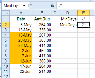
Do you use Excel to keep track of upcoming payments, or other dates? To make that list more helpful, you can highlight upcoming dates in Excel. In this example, we’ll highlight dates if they’re within the next couple of weeks.
Add Products to Excel Order Form
 The summer is off to a good start here in Canada – we had perfect weather for our first long weekend of the season. My garden is almost ready, and I haven’t killed any of the plants yet!
Over the weekend, my Contextures website and blog were moved to a different web host and servers. It seems to have gone smoothly, but please let me know if you see anything strange. Well, stranger than usual. 😉
Click to Add Products to an Order
As you know, when you’re moving, you sometimes find interesting things in the back of the closet. While I was checking the website, I found this sample file, that lets you click to add products to an Excel order form.
On the Data Entry sheet, you can select a product category, from the drop down list.

When a category is selected, the Excel Worksheet_Change event code runs, and lists all the products in the selected category.
Worksheet Change VBA Code
The code uses an Advanced Filter to copy the products onto the Data Entry sheet.

In the list of products, click on any row, in column G, to add that product to the order form.

The Order Form Move Code
Another event code runs when you click on a cell in column G – the SelectionChange event.
It checks the column and row number of the cell that was selected, and checks for an entry in column A.

If the selection was in column G and the row number is greater than 6, and there is something in column A, an X is added to the cell.
Then, the MoveRow code runs, and it copies the selected row to the order form, in the row below the previous product ordered.

Here is the OrderForm sheet, with condiments and dairy products listed.

Future Enhancements to the Product List Order Code
When you go back an look at an Excel project, you can usually think of several things that would improve it. In this example, I’d like to add code that prints the completed order form, and clears the OrderForm sheet.
Is there anything else that you’d add or change?
Download the Product List Order Workbook
To download the product list order form workbook, you can visit the Sample Files page on the Contextures website. In the Filters section, look for FL0016 – Move Items to Order Form.
The file is in Excel 2003 format, and zipped. It contains macros, so enable those, if you want to test the code.
Another Excel Order Form
To see another example of an Excel order form, go to the Excel Order Form page on my Contextures site.
In the video below, I give a quick demo of how that order form works.
_________________
Your Excel Spreadsheet Smells
Do your spreadsheets smell? This week, a tweet from Felienne Hermans caught my eye.
- “Our @icse2012 paper on spreadsheet smells already has a citation before publication”
Spreadsheet smells? I’ve seen some stinky spreadsheets, but have never read a conference paper on spreadsheet smells.
It sounded intriguing, so I followed the link to Felienne’s paper – Detecting and Visualizing Inter-worksheet Smells in Spreadsheets.
Code Smells
The starting point for the paper is the code smell metaphor introduced in Martin Fowler’s book, Refactoring: Improving the Design of Existing Code.
I don’t have that book, so I visited Wikipedia, to see what it knew about code smells.
Wikipedia Code Smells
Fortunately, Wikipedia had a helpful summary of common code smells, and I’ve listed a few of them below. Can you see how these code smells relate to Excel, whether you’re building worksheets, or creating Excel VBA code?
- Duplicated code: identical or very similar code exists in more than one location.
- Long method: a method, function, or procedure that has grown too large.
- Contrived complexity: forced usage of overly complicated design patterns where simpler design would suffice.
- Excessive use of literals: these should be coded as named constants, to improve readability and to avoid programming errors.
Hmmm…replace “code” with formulas, and you’ve probably seen (or created) workbooks that had those code smells.
I’ve been guilty of creating some of those smells, and have seen workbooks start small, and slowly grow out of control.
Spreadsheet Smells
Among the most frequent spreadsheet smells that Felienne and her colleagues found were:
- Inappropriate Intimacy – a worksheet that is overly related to a second worksheet.
- Feature Envy – if there is a formula that is more interested in cells from another worksheet, it would be better to move the formula to that worksheet
- Shotgun Surgery – a formula F that is referred to by many different formulas in different worksheets…chances are high that many of the formulas that refer to F will have to be changed if F is changed.
Read More About It
If you’d like to learn more about spreadsheet code smells, take a look at the Spreadsheet Smells paper written by Felienne and her colleagues, to see how their research was done, and what their conclusions were.
You can also read other papers that Felienne has written on this topic, if you’d like to learn more: Felienne Hermans Publications
Have you read anything similar, or heard about code smells before?
_______________
Excel Pivot Table Selection Quick Tip
To format a pivot table, you can select a specific section, such as one of the fields, or a grand total. When you point to a field heading, a black arrow will appear, if the Enable Selection setting is turned on.
Black Arrow Pointer
In the screen shot below, you can see the black arrow at the top of the Product field. Click in that spot, and all the Product item labels are selected.

Click in that spot again, and the Product heading is selected, instead of the item labels.

Pivot Table Field Setting Quick Tip
Instead of a single click on a heading cell, you can point to an outer field heading and double-click when the black arrow appears.
In the screen shot below, the black arrow is on the Bran product heading cell.
Note: This trick won’t work on an inner field, like Region, which has no other fields under it.

Open Field Settings
Double-click on the outer field heading, and the Field Settings dialog box opens.
In there, you can change the layout and other settings, and add or remove subtotals.

Right-Click Menu
Another way to open the Field Settings dialog box is to right-click on an item, and click Field Settings in the popup menu. This works for both inner and outer fields in the pivot table.

I find the double-click shortcut to be quicker and easier – as long as you remember to point somewhere that the black arrow appears.
Watch the Pivot Table Selection Video
To see the steps for selecting section of an Excel Pivot Table, you can watch this short video tutorial.
_________________
Show Data From Hidden Rows in Excel Chart

You can add a chart in Excel, based on worksheet data, but if you filter the data, and rows are hidden, that data also disappears from the chart. See how to prevent that problem from happening.
Continue reading “Show Data From Hidden Rows in Excel Chart”
Add New ComboBox Items in Excel UserForm
If you want to enter data in an Excel worksheet, while keeping the data sheet hidden, you can create an Excel UserForm.
I’ve updated my sample file, so you can now add new parts to the drop down list, while you’re entering data. It’s almost working the way it should, but I’m stuck on one step, so if you have a solution, please let me know!
[Update: Problem solved with a workaround — see below.]
Select Part from ComboBox Drop Down List
In the sample file, you can click the Add Parts Information button on the worksheet, to open the UserForm.
Then, at the top of the UserForm, select a Part ID from the combo box drop down list.
The drop down list shows part ID, and the part name. After you make a selection, only the part ID appears in the combo box.

The Parts List
On another sheet in the workbook, there are two lists – Location, and Parts. These are dynamic named ranges, based on a formula, and the named ranges will expand automatically, as new items are added to the lists.

Add a New Part to the List
In the latest version of the sample file, you can add new parts to the list, while you are entering data in the UserForm.
- First, if the Part ID that you want is not in the list, type it into the Part ID combo box.
- Next, when you press the Tab key, to move to the next control, a Part Description text box will appear.
- Enter the description, then fill in the rest of the data.
- Finally, click the Add This Part button

Select the New Part
After you click the Add This Part button, the new item is added to the Parts List, and the Parts list on the worksheet is sorted A-Z, based on the PartID column.

The next time you click the Part ID combo box arrow, you will see that the new item now appears in the drop down list.

SetFocus Problem
My goal was to have the Part Description activated, as soon as it was made visible. However, the VBA code wouldn’t cooperate, so I’ve commented out the following line in the code:
Me.txtPartDesc.SetFocus
If you have a solution for getting that line to work, please share it in the comments, or send me an email. I’d appreciate it!
Set Focus Workaround
Update: Thanks to JeanMarc, Jon and Dave, the tab order is working now. You can see their suggestions in the comments below.
- Instead of being hidden, the Parts Description textbox moves to the far right, so it’s not in the visible part of the form, then moves back when needed.
- To keep the tab key from stopping on the “off form” textbox, its position is checked. If the textbox is at the far right, go to the next control.
Download the Sample File
To get the sample file, and to check the Excel VBA code, you can download the file from my Contextures website.
On the Sample Excel Files page, in the UserForm section, look for UF0017 – Parts Database with Updateable Comboboxes
The file is available in Excel xlsm or Excel xls format, and zipped. The workbook contains macros, so enable those if you want to test the UserForm combo box code.
_____________________