Split Text Into Columns in Excel-Get Specific Column

If you had to split a text string into separate columns in Excel, how would you do that? There are built-in tools that could help you, and Excel functions and formulas will do the job too. If your version of Excel has the latest functions and features, there are fancy new text functions for you to try.

Comma-Separated Text

In the screen shot below, there’s an Excel worksheet, with a list of items that were sold, in column A.

Each cell has a comma-separated item description, with 3 pieces of information:

Product Code
Product Name
Product Size

Split Text with Excel Tools

You could quickly split that product description into multiple columns, using Flash Fill, or Text to Columns, if it’s just a one-time thing.

This animated gif shows the steps for splitting a different data set with Flash Fill.

Tip: To save time, use the Flash Fill shortcut – Ctrl + E

Excel Formulas – All Versions

In some workbooks, you might prefer to split the data by using formula, so the separated data updates, if the original text string changes.

No matter what version of Excel you’re using, you can create formulas that split the text string into separate columns, based on those comma separators.

Most formula solutions use a combination of Excel text functions, like FIND, LEFT, MID, and RIGHT.

There are formula examples on the Split Address Formulas page on my Contextures site.

One example has comma-separated text strings
Another example has a variety of separators, and that makes the task more challenging!

Excel 365 Formulas

If you’re lucky enough to have an Excel version that includes the latest features and functions, you can use simpler formulas to separate the parts in a text string.

The 3 latest text functions are TEXTBEFORE, TEXTAFTER, and TEXTSPLIT.

To separate the item descriptions in the example below, I used the TEXTSPLIT function, with this formula in cell B4:

=TEXTSPLIT(A4, “, “)

Then, copy that formula down, to the last row of data.

Because there are 3 parts in the text string, Excel shows the formula results in 3 separate columns.

When cell B4 is selected, the thin blue border shows that the formula results have spilled into columns C (Item) and D (Size)

Problems in Excel Table

Usually, I keep lists in a named Excel table, because that makes it easier to work with the data. There are built-in filters, and other handy features.

However, Excel tables don’t play nicely with formulas that spill into adjacent cells.

As you can see in the screen shot below, instead of showing the results, the formula cells show a #SPILL! error.

Avoid Excel Table Problem

If you need to keep your data in a named Excel table, but you also want to use the new TEXTSPLIT function, here’s one way to avoid the #SPILL! error problem.

Instead of using TEXTSPLIT on its own, combine it with another new Excel function – CHOOSECOLS.

Tip: To see which Excel versions include this function, go to the CHOOSECOLS page on the Microsoft site, and click the drop-down list for Availability.

With the CHOOSECOLS function, you can tell Excel to return one or more specific columns from an array.

=CHOOSECOLS(array, col_num1, [col_num2],…)

The TEXTSPLIT function will create the array, in this example, and we’ll put the column number in a worksheet cell

Which Columns to Return

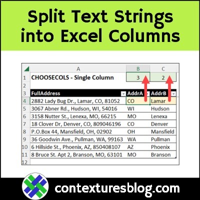
In the next example, shown in the screen shot below, there are comma-separated addresses in column A. Each address has four parts:

Street, City, State, Zip Code

The list is in a named Excel table, so I can’t use a TEXTSPLIT formula on its own – that would result in a #SPILL! error.

Instead, I’ll use CHOOSECOLS to get a single column from the full address.

First, I typed column numbers in cells B1 and C1:

Cell B1: Number 3 – State is the 3rd part of the full address
Cell C1: Number 2 – City is the 2nd part of the full address

Enter the Formulas

Next, I entered this formula in cell B4, to get the State code:

=CHOOSECOLS(TEXTSPLIT([@FullAddress],”, “),B$1)

The formula fills down automatically, because the list is in a named Excel table

After that, I entered this formula in cell C4, to get the City Name:

=CHOOSECOLS(TEXTSPLIT([@FullAddress],”, “),C$1)

Again, the formula fills down automatically, because the list is in a named Excel table

Choose Different Columns

Because the column numbers are entered on the worksheet, its easy to change the formula results, to show a different part of the full address.

Just type any number between 1 and 4 in cells B1 and C1, to see the results for that column number.

But, if you type an invalid number, the formula will return a #VALUE! error.

Tip: To avoid that problem, you could create data validation drop down lists in cells B1 and C1, instead of allowing invalid entries.

_________________________