Excel Drop Down List with Latest Items at Top

In this data validation drop down list, the most recently ordered products are at the top. The rest of the product names are below those, in alphabetical order. There’s a worksheet cell where you can set the number of top items. This technique uses new functions, SORTBY and MAXIFS, which are available in Excel 365.

Latest Items at Top

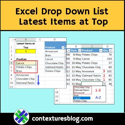
Here’s what the drop down looks like, in the Product column on the Orders worksheet.

• The 3 latest product names at the top
• All other products are below, listed A to Z

Product List Table

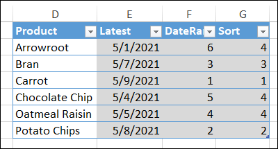
In the sample workbook, one a sheet named Lists, there is a named Excel table with product names, and 3 columns with formulas.

How Many Top Items?

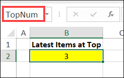
On the same worksheet as the product table, there’s a cell named TopNum.

In that cell (B2), type the number of top items that you want to show in the drop down list.

For example, type 3 in the TopNum cell, and:

• The 3 most recently ordered products will be at the top of the drop down list
• All other products are below, listed A to Z

Latest Date Formula

To calculate the latest date that each product was ordered, this MAXIFS formula, in the Latest column, checks the Orders table (SalesData).

• =MAXIFS(SalesData[Date], SalesData[Product], [@Product])

NOTE: You can read more about MAXIFS on the Microsoft site. That page explains how the function works, and shows 6 examples of how to use it.

DateRank Formula

There’s a simple RANK formula in the DateRank column:

• =RANK([@Latest],[Latest],0)

See more RANK examples on my Contextures site.

Sort Formula

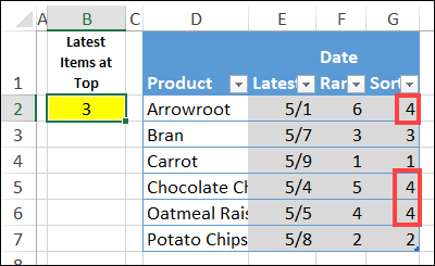
The final column, Sort, returns a number that’s used for the first sort – top items or “all other”

• =IF([@DateRank]<=TopNum,[@DateRank],$B$2+1)

Make the Sorted Product List

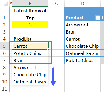
The List sheet also has a spill formula (Excel 365), in cell B5,  to create the sorted product list. The products are sorted by the Sort number, and then by product name.

• =SORTBY(tblProd[Product], tblProd[Sort],1, tblProd[Product],1)

ProdList Named Range

The product list is used for a data validation drop down, on the Orders sheet.

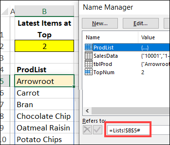
To make it easy to refer to the list, a name, ProdList, was created, using the spill operator (#).

• ProdList: =Lists!$B$5#

You can see the name and its formula in the Name Manager, and learn more about named ranges on my Contextures site.

Create the Drop Down List

On the Orders sheet, there’s a data validation drop down list in the Product column.

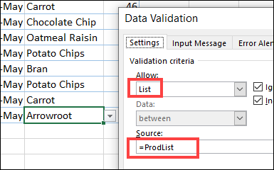
When you select a cell in the Product column, the drop down arrow appears.

Select one of the recently-ordered products, or find a product name in the A-Z section.

Get the Sample File

To get the Latest Items at top of List sample file, go to the Latest Used Items at Top page on my Contextures site.

That page also has details on the product table formulas, and how to set up the data validation drop down list.

The zipped Excel file is in xlsx format and does not contain any macros.

____________________________

Excel Drop Down List with Latest Items at Top

__________________________