Sometimes, a MATCH formula returns an #N/A error, even if the value you’re looking for is in the lookup table. The reason for that could be numbers that Excel sees as text, and here are a couple of ways to fix that problem. And if numbers aren’t the problem, I’ve got a couple of other things to check too!
MATCH Function Examples
Before we start troubleshooting the MATCH function, here’s a short video that shows how the function works. It has four MATCH examples, so you can see different ways to use it.
There are more examples on the INDEX and MATCH page of my Contextures site.
Numbers or Text
And now, let’s do some MATCH troubleshooting.
One common cause for a MATCH function error is trying to match:
- real numbers in one place
- text “numbers” in another place
Excel sees those as completely different things, even if they look the same on the worksheet, so they don’t “MATCH”.
This video shows the steps for fixing those text/number problems, and there are written steps below.
Video Timeline
- 00:00 Introduction
- 00:23 MATCH Error
- 00:58 Number or Text
- 01:46 Fix the Error
- 02:21 Minus Signs
- 02:51 Other Formulas
- 03:31 Match Numbers to Text
- 04:34 Get the Workbook
Not Real Numbers
For example, your lookup table might have “numbers” that are really text.
How can you tell?
- If you select one, and look in the formula bar, there might be an apostrophe at the start of the cell
- If you select two or more, and look in the Status bar, there is a Count, but no Sum showing
- If you use the SUM function for those cells, the total is zero
MATCH Function Error
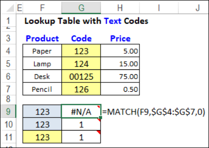
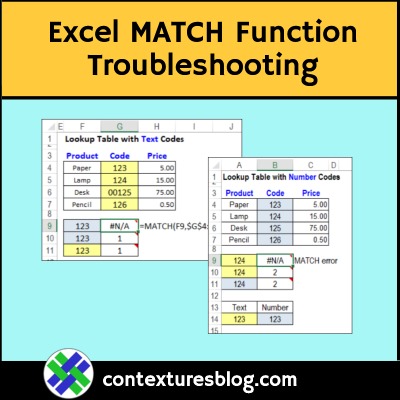
In this screen shot, the yellow cells contain text, and the blue cells have real numbers.
The MATCH formula in cell G9 has an error result, because the real number, in cell F9, doesn’t match the text number 123, in the lookup table, cell G4.
- =MATCH(F9,$G$4:$G$7,0)
Fix the Data
One way to fix the problem is to change the text numbers to real numbers, if you’re able to do that.
There are a few ways to do that, so check the suggestions on my Contextures site.
This video shows one way to convert text to numbers – using Paste Special
Change the MATCH Formula
If you can’t change the data to real numbers, another option is to change the MATCH formula.
Here’s the original MATCH formula in cell G9, that returns an error.
- =MATCH(F9,$G$4:$G$7,0)
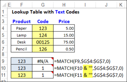
To fix the problem, add an empty string (“”) in the formula, after the lookup value. That changes a real number to a text number, so it will find a match in the lookup table.
Here is the formula in cell G10, where F10 is a number, and the MATCH formula works correctly:
- =MATCH(F10 & “”,$G$4:$G$7,0)
NOTE: The revised formula also works for cells that contain text numbers, like the one in cell F11.
Lookup Table With Real Numbers
How can you fix the opposite problem – a lookup table with real numbers, and a text number to find?
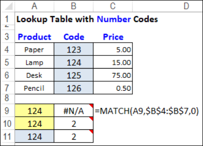
Here’s an example, with numbers in the blue cells, and text in the yellow cells.
The MATCH formula in cell B9 returns an error, because A9 has text, and the lookup table has numbers (B4:B7).
- =MATCH(A9,$B$4:$B$7,0)
Fix the MATCH Formula for Numbers
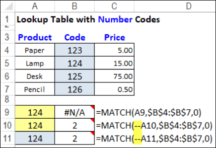
To fix this type of problem, type two minus signs in the formula, before the lookup value. That changes a text number to a real number, so Excel can find a match.
Here’s the formula in cell B10, where A10 is text, and the MATCH function works correctly:
- =MATCH(–A10,$B$4:$B$7,0)
NOTE: The revised formula also works for cells that contain real numbers, like the one in cell F11.
Another MATCH Problem
If numbers aren’t the problem with your MATCH function, check for extra space characters:
- One of the values might have leading spaces (or trailing, or embedded spaces)
- The other value doesn’t have those space characters
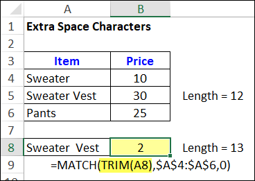
If that’s the problem, and you can’t remove the spaces, use the TRIM function with MATCH. That removes any leading, trailing and duplicate spaces.
- =MATCH(TRIM(A8),$A$4:$A$6,0)
That fixed the problem in cell B8, where the item name in cell A8 had an extra space between the words.
Get the Sample File
To get the MATCH function sample workbook, and one more MATCH troubleshooting tip, go to the INDEX and MATCH page on my Contextures site.
In the Download section there, get the first file – INDEX/MATCH Examples. The workbook is in xlsx format, and doesn’t contain any macros
____________________________
Excel MATCH Function Error Troubleshooting Examples
____________________________

Wow, finally found a simple solution. Great article, many, many thanks!
thank you so much, I finally fixed the problem.
I am just wondering why changing format cell in excel doesn’t work, and I had to match format manually by using (– or $””)/