
December is only 2 days away, so it’s time for an Excel Advent Calendar! I’ve made two new versions this year, and they don’t use macros, just basic Excel features. Even if you don’t need an Advent calendar, take a look to see how they’re set up . You might find a use for these techniques in other projects.
Fancy Calendars
When our kids were young, they got an Advent Calendar every December, with 24 numbered doors, and a small chocolate treat behind each door.
In past years, I’ve shared Excel Advent calendars with Christmas pictures instead of chocolate. Those calendars had macros, to show each day’s “treat”.
For example, the 2009 version had shapes to click, and a macro changed the shape’s colour to “No Fill”. That revealed the picture behind the shape.
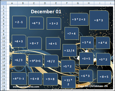
In 2010, the Excel Advent Calendar looked a bit different, and you had to solve a formula to find the right door number. The shapes and pictures worked like the 2009 version.
Keep It Simple
Unlike those fancy versions, this year’s Advent calendar is simple, with no macros — just formulas and conditional formatting. It’s always full to see what Excel can do with just its basic features.
The calendar is in a 6 x 4 grid of cells, numbered from 1 to 24. Each day, the next number changes to a picture automatically – you don’t have to click anything.

Create a Background Picture
Instead of using a random layout for the pictures, I created an image with the Advent calendar “treats” carefully lined up.

If you put an image on a worksheet, it’s on top of the cells, and covers everything up. I needed the image behind the cells, for this no-macro Excel Advent calendar to work.
So, instead of inserting the image on the sheet, I went to the Page Layout tab on the Excel Ribbon, and click the Background command. Then I selected my calendar grid image to use as the worksheet’s background.

Cover the Background
When you add a Background image, you don’t just get one copy of it. No, you get an entire worksheet with the image repeated!
To fix that problem, and end up with only one visible image, I followed these steps:
- First, adjust the column and row widths for the 6 x 4 grid, to line up with the grid in the background image
- Then, select all the cells, and use a fill colour to cover the background (I used dark blue)
- Finally, select the cells in the 6 x 4 grid, and change them to No Fill
Admin_Dates Sheet
There’s another sheet in the Advent Calendar workbook – Admin_Dates. It helps with the formatting and formulas.
At the top of the sheet, there are formulas to calculate the current day and month, and yellow cells where you can enter a different date, for testing.
Three of the cells are named:
- Cell C2 is named CurrMth
- D2 is named CurrDay
- F2 is named AdvMth
There is also a 6×4 grid with numbers for the Calendar sheet.

Add the Numbers
The Advent calendar has 24 doors (cells). Each door should show a number, until its day arrives. After that, it should show a Christmas picture.
To make the numbers stand out, I used Calibri, Bold, 36, centred horizontally and vertically.
To show or hide the number without macros, I used a formula in each cell, linking to the 6×4 grid on the Admin_Dates sheet.
Here is the formula from cell B4, the first cell in the Advent Calendar grid. It refers to cell B10 on the Admin_Dates sheet, where the Days Grid starts.
=IF(CurrMth<>AdvMth, Admin_Dates!B10, IF(CurrDay <Admin_Dates!B10, Admin_Dates!B10, “”))

- If the current month isn’t December (AdvMth=12), show the cell’s number, from the reference grid on the Admin_Dates sheet.
- If the current day number is less than then day number in the reference grid, show the cell’s number
- Otherwise, show an empty string (“”), so we can see the picture.
Add Conditional Formatting
You should only be able to see the Advent calendar “treats” when you reach that day of the month. Before that, the picture should be hidden.
The calendar grid has No Fill, and I added Conditional Formatting to show a green fill colour, when the cell contains a number.
To add the conditional formatting:
- Select cell B4:G7 (the calendar grid cells)
- On the Home tab of the Excel Ribbon, click Conditional Formatting, and click New Rule
- In the Select a Rule Type section, choose Use a Formula to determine which cells to format
- In the formula box, type this rule, referring to the active cell (B4): =B4<>””
- Click the Format button, and on the Fill tab, choose Green as the fill colour.
- Click OK, twice, to apply the Conditional Format

The formula checks the cell, to see if it contains an empty string. If not, the conditional formatting will be applied, and the cell will have green fill.
The Background Image
Here’s how I made the image for the background, in case you’re interested.
- First, I set up the worksheet, with the heading rows, and the calendar grid cells the approximate size that I wanted them.
- Next, I took a screen shot with Snagit, and checked its size in Windows Explorer.
- Then I uploaded that screen shot to Stencil, which I use to make graphics.
- I made a new image, with my screen shot as a background, set for its size
- Then I searched for Christmas icons, and put one into each square, resizing each one to fit.
- Finally, I downloaded the image in png format, to keep it as small as possible.

The WingDings Advent Calendar
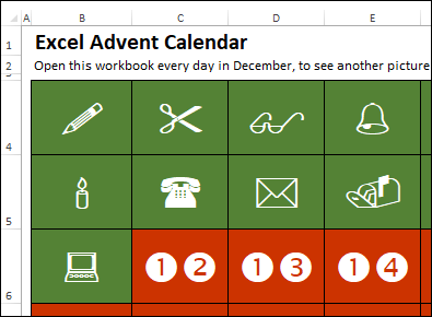
If that background image Excel Advent calendar is too fancy for you, there’s good news! I made another no-macros Advent Calendar this year, and it’s an even smaller, plainer file. Instead of a background picture, the “treats” are created with a font.
The main page uses Wingdings font, because it has both numbers and pictures. (WingDings 2 is similar). And yes, most of the images are from the 1950s, but your kids will have fun guessing what they are!
On another sheet, the CHAR Function pulls the number and picture options for each square, based on the character numbers. This formula is in cell C3, to create the one or two digit number.
=CHAR(D3)&IFERROR(CHAR(E3),””)
Then, the calendar shows the number or picture, depending on the current date. This formula is in cell B3, the Show column.
=IF(CurrMth<>AdvMth,[@Num],IF(CurrDay<A3,[@Num],[@Pic]))
- If the current month (CurrMth) is not 12 (AdvMth), result is number from column C (@Num)
- If the current day (CurrDay) is less than the value in column A, result is number from column C (@Num)
- Otherwise, result is picture from column F (@Pic)

Excel Advent Calendar Downloads
To get these Excel Advent Calendars, and see how they work, go to the Excel Advent Calendar page on my Contextures site.
That page has download links for these “no macros” Advent calendars, and for the previous versions, which do have macros.
Even if you don’t need an Advent calendar, you might find some useful techniques for your other Excel projects
___________________

_______________