To make a chart right in the worksheet cells, use Excel Data Bars, built with conditional formatting. See how to add a standard set of Data Bars (Excel 2007 and later), and adjust their settings to make the bars look better.
And remember to mark your calendars – next Tuesday, October 17th, is Spreadsheet Day – alert your family and friends!
Add Excel Data Bars
First, to add a standard set of Data Bars , follow these steps:
- Select the cells with numbers (don’t include any row or column totals).
- On the Ribbon’s Home tab, click Conditional Formatting.
- Click Data Bars, and then click any one of the Data Bar options
NOTE: You can change the Fill Style (gradient or solid) later, or choose a different colour for the Data Bars.

The selected cells will show Excel Data Bars, along with the original numbers. In the screen shot below, the Green Gradient data bar option was selected

Change the Data Bar Settings
After you add the Data Bars, you can make a few changes to the default settings, to make the bars look better. Here are the steps for opening the Settings dialog box:
- Select the cells that contain the data bars.
- On the Ribbon, click the Home tab
- In the Styles group, click Conditional Formatting, and then click Manage Rules.
- In the list of rules, click your Data Bar rule.
- Click the Edit Rule button, to open the Edit Formatting Rule dialog box.
Hide the Numbers
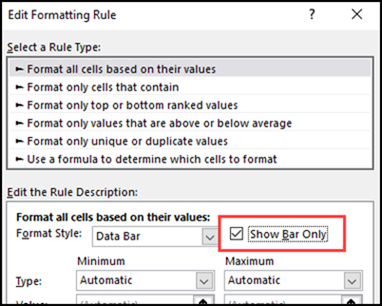
You won’t make any changes in the “Select a Rule Type” at the top. Look at the settings in the lower section – “Edit the Rule Description”.
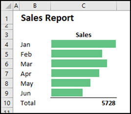
One simple tweak is to hide the cells’ numbers. This could be useful if you want people to focus on the “big picture”, rather than the details.
- To hide the numbers, add a check mark to “Show Bar Only”
- Then, click OK, to see the revised Data Bars.
Change Excel Data Bar Appearance
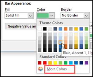
Another easy change is to select different options in the “Bar Appearance” section.
- The Fill can be Gradient or Solid, and you can pick a colour from the standard palette, or from the “More Colors” screen.
- The Border can be Solid, with any colour choice, or choose No Border
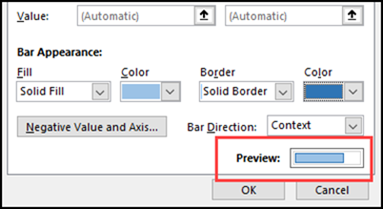
- A Preview, at the bottom right of the dialog box, shows what the revised Data Bars will look like.
- When you’re happy with the appearance, click OK
Data Bar Minimum
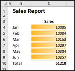
You can also change the Minimum and Maximum settings for the set of Data Bars. By default, both are set to “Automatic”. From my experience, that results in a Minimum of zero, and a Maximum of the highest value.
The Automatic settings are fine for some data, but you can change them. For example, if there is only a small difference among the numbers, as in the screen shot below, you might want to highlight that differences.
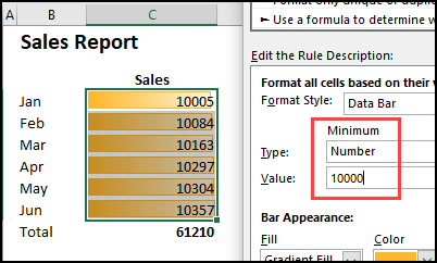
To focus on the differences in this example, change the minimum setting.
- Open the Edit Rule dialog box
- For Minimum, click the Type arrow, and choose Number
- In the Value box, type 10000
- Click OK, to close the dialog box
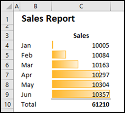
The Data Bars change – range is only 357, instead of 10357. so you can clearly see the small difference among the numbers.
NOTE: Using a hard-coded value of 10000 worked well in this case, but hard coding wouldn’t be a good solution if the numbers will change. See the next section for another option.
Data Bar Maximum
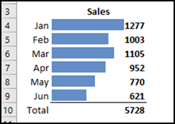
If you use the default Maximum setting, the bar for the highest value fills the cell. If the numbers are showing, and the bars have a dark fill colour, it will be difficult to read some of the numbers
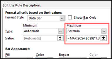
To fix that problem, change the Maximum, to leave a space at the right end of the bar. Instead of hard-coding a Maximum value, we’ll use a flexible solution.
- Open the Edit Rule dialog box
- For Maximum, click the Type arrow, and choose Formula
- In the Value box, type this formula: =MAX($G$4:$G$9)*1.3
- Click OK, to see the result
The MAX function finds the highest number in the range of cells, and that amount is multiplied by 1.3. That creates enough space for the numbers at the right of the cell.
Use a Cell Reference
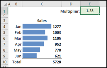
For even more flexibility in the Maximum setting, enter the multiplier in a worksheet cell, then refer to that cell in the Data Bars Maximum formula.
In the screen shot below, the multiplier is in cell E1 – you could use a cell on a different sheet, if you prefer.
The formula for this Maximum s: =MAX($C$4:$C$9)*$E$1
Then, if you need a little more space for the numbers, increase the multiplier in cell E1. That’s quicker than going back into the Edit Rules dialog box.
Video: Excel Data Bars
This video shows how to set up Excel Data Bars, and change their default settings.
Download the Sample File
Learn more about Excel Data Bars on my Contextures website, and download the sample file on that page, to see how they work.
_________________________

Hi,
I am using data bars to show cell value that can range from 0 to 1. I want the bar to be green when between 0 and 1 values. The numbers indicate stress level. Anything between 0 and 1 is OK, anything above 1 is no good. ie. 0.5 stress is OK, 1.5 not OK.
So I want green data bars for values between 0 and 1, and solid red for values greater than 1. Right now the bars are working OK for between 0 and 1, but above 1 it shows solid green. I would think that above 1 value would not trigger the formatting. Any suggestions?
If you are showing the data bar in a different cell, you can make it so that the good values are positive and the bad values are negative. Adjust the Minimum and maximum to accommodate for the values that you want. It will automatically place a bar midline that you can update to not show if you prefer. If it is a good value it will go to the right of the midline and be in green. If it is a negative value it will be to the left of the midline and will default to red, which you can change to a differnt color like white if you prefer.