Highlight Cells Based on Two Conditions

Happy New Year! I hope you had time to relax over the holidays, and you stepped away from the computer for a while. Unless you were using the computer as excuse to hide away from all the holiday chaos! Now we’re back to work, and one of the first questions I got this year was how to highlight cells based on two conditions.

Turn Cells Red

The person who sent the question wanted to highlight cells based on 2 conditions:

1. The country code “US”  is entered in cell B2.
2. The data entry cell contains “United States”

Here’s what the worksheet looks like, after that conditional formatting is set up in cells D5:D14

Enter the 2 Conditions

There isn’t a built-in conditional formatting rule that will do this. We’ll need to set up a special rule for this, using a formula.

In that formula, you could hard-code the “US” and “United States” conditions. However, I like to put the conditions in worksheet cells instead, so it’s easy to see them, and change the conditions later, if you need to.

In this workbook, the conditions are in cells E2 and F2, on the same sheet as the data entry cells. You could put them on a different sheet, if you prefer, to prevent people from accidentally changing them. You could also name the cells, and use those names in the conditional formatting formula.

Add the Country Code Cell

People will type a country code in cell B2, so I filled that cell with yellow, to make it stand out. For testing, I put “US” in that cell.

Add the Conditional Formatting

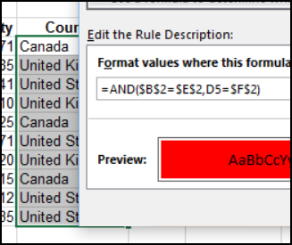
The next step is to add conditional formatting to the country cells in the data range  D5:D14. We’ll use the AND function, to check both conditions, and the formula is explained in the next section.

• Select cells D5:D14, where the country names are listed for the orders
• On the Ribbon’s Home tab, click Conditional Formatting, then click New Rule
• Click Use a Formula to Determine Which Cells to Format
• For the formula, enter    =AND($B$2=$E$2,D5=$F$2)
• Click the Format button.
• Select red as the fill colour, and click OK

•   Click OK, to apply the conditional formatting

Cells Are Highlighted

Because “US” is entered in cell B2, any cell in D5:D14 that contains “United States” is coloured red.

How the Formula Works

The conditional formatting formula is: =AND($B$2=$E$2,D5=$F$2)

The AND function checks the 2 conditions:

1. Does cell B2 match the condition entered in cell E2
2. Does the data entry cell (D5) match the condition entered in cell F2

Cell D5 is used in the formula, because that was the active cell when the conditional formatting was applied.

Some of the references are Absolute, and one is Relative:

• Absolute references are used for $B$2, $E$2 and $F$2 because no matter where the conditional formatting is applied, it should always check those cells.
• A relative reference is used for the data entry cell (D5), because it should adjust to match each cell where the conditional formatting is applied.

Get the Sample File

To see how this conditional formatting works, you can download the sample file. Go to the Conditional Formatting Examples page on my Contextures website. Scroll down to the Download section, and click the link to get the workbook.

The zipped file is in xlsx format (or xls format for Excel 2003), and does not contain any macros.

_________________