
Is there a harder working team in Excel, than the reliable duo of INDEX and MATCH? These functions work beautifully together, with MATCH identifying the location of an item, and INDEX pulling the results out from the murky depths of data. See how to find text with INDEX and MATCH.
Find Text in a String
Last week, Jodie asked if I could help with a problem, and INDEX and MATCH came to the rescue again.
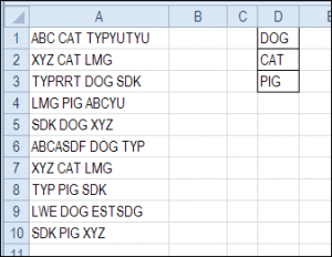
Jodie sent me a picture of her worksheet, with text strings in column A and codes in column D. Each text string contained one of the codes, and Jodie wanted that code to appear in column B.
Would you use INDEX and MATCH to find the code, or another method? Keep reading to see my solution, and please share your ideas, if you have other ways to solve this.

Count the Occurrences With COUNTIF
When you want to find text that’s buried somewhere in a string, the * wildcard character is useful. We can use the wildcard with COUNTIF, to see if the string is found somewhere in the text.
I entered this test formula in cell B1. This formula needs to be array-entered, so press Ctrl + Shift + Enter.
=COUNTIF(A1,”*” & $D$1:$D$3 & “*”)

There are wildcard characters before and after the cell references to D1:D3, so the text will be found anywhere within the text string.
To see the results of the array formula, click in the formula bar, and press the F9 key. The array shows 0;1;0 so it found a match for CAT, which is in the second cell in the range, $D$1:$D$3.
- Important: After you check the results, press the Esc key, to exit the formula without saving the calculated results.

Get the Position With MATCH
Next, you can add the MATCH function, wrapped around the COUNTIF formula, to get the position of the “1” in the results.
Make the following change to the formula in cell B1, and remember to press Ctrl + Shift + Enter.
=MATCH(1,COUNTIF(A1,”*”&$D$1:$D$3&”*”),0)

The result is 2, so the code “CAT”, the 2nd item in range D1:D3, was found in cell A1.
Get the Code With INDEX
Next, the INDEX function can return the code from the range $D$1:$D$3, that is at the position that the MATCH function identified.
Make the following change to the formula in cell B1, and remember to press Ctrl + Shift + Enter.
=INDEX($D$1:$D$3,MATCH(1,COUNTIF(A1,”*”&$D$1:$D$3&”*”),0))

The result is CAT, so the formula is working correctly.
Prevent Error Results With IFERROR
There should be one valid code in each text string, but sometimes the data doesn’t cooperate. Just in case there are text strings without a code, or more than one instance of the code, you can use IFERROR to show an empty string, instead of an error. (Excel 2007 and later versions)
=IFERROR(INDEX($D$1:$D$3,MATCH(1,COUNTIF(A1,”*”&$D$1:$D$3&”*”),0)),””)
Enter with Ctrl + Shift + Enter, and then copy the formula down to row 10.

In cell B6, the formula returns an empty string, and the cell looks blank, because none of the valid codes are in the text that’s in cell A6.
Use a Named Range
Instead of referring to range $D$1:$D$3, you could name that range, and use the name in the INDEX/MATCH formula. That would make it easier to maintain, if the size of the codes list will change.

Download Find Text With INDEX and MATCH Sample File
To get the sample file, and see how the formula works, go to the INDEX and MATCH page on my Contextures site.
In the Download section on that page, look for sample file 4 – Find Text From Code List. The zipped file is in xlsx format, and does not contain macros.
More INDEX and MATCH Examples
There are more examples of using INDEX and MATCH on my Contextures site.
For example, this video shows how to use INDEX and MATCH to find the best price.
____________________________
Hello Debra,
I have been using the code for the VLookupInvMark.xls, thank you.
I now need the same output but when I Type an X in column J (so data is to the left).
Can you help?
Hello Debra,
This is a great post! I was fortunate enough to come across this reading to help me construct my own Excel template. I have followed your code {=IFERROR(INDEX(CodeList,MATCH(1,COUNTIF(A1,”*”&CodeList&”*”),0)),””)}, and the formula does exactly as you have explained in your article. However, there is one problem I came across with the formula in the spreadsheet that I’m working on. When there is a blank field located in the middle of the list, the function does not account for the texts listed below. For example, when the text “CAT” is taken out from your codelist, the text “PIG” is no longer displayed in the column B. This is where I’m stuck. If you know how to solve this problem and provide me with the formula, I’d highly appreciate it.
Thank you
🙂
I have used this formula to search multiple texts in a cell.
Search list contains several texts having few common texts within them e.g. “PB 15” and “PB 15:2”.
This formula returns “PB 15” while searching for “PB 15:2” also.
could you kindly inform if it could be restricted to exact match, in this case “PB 15:2”.
thanks for the help..
According to your question, a simple solution is to place PB 15:2 above PB 15 on the list. This answers your post, but you have to go through the trouble of listing the names above or below something else.
Thank you, Andy.
But the list I am searching is too long (50K rows). Hence need some auto solution please..
Ganesh,
You can create a table to your list of 50k rows. After you have done so, you can arrange the names via sorting z to a using the table options. This should give PB15:2 above PB15.
Hello, hope you don’t mind me asking but I was wondering you could help. I’m trying to set up a spreadsheet which is linked to a diary system (all excel) what I’m trying to do with the linked spreadsheet is for it to show “booked” when any text is shown in a particular cell from the diary. I want to put the codes in for each day, so 1st July = if something (any text) is in the diary it says “booked” if no text it says “available”.
Have you got an idea of how to do this??
Jemma,
You may use a combination of If and Counta functions to respond if the chosen spreadsheet contains any non-blank cells.
Let’s assume we have two different spreadsheets “A” and “B”
When this code is used in Spreadsheet “A” in cell A1, you can find out whether anything is written in the spreadsheet “B”
=If(Counta([B.xlsx]Sheet1$1:$1038576)>0,”Booked”,”Available”)
*Counta formula responds with a number count of any non-blank cells.
*When counta formula responds with a # greater than 0, that means that there is something written in the spreadsheet vs. 0, which would mean that there isn’t anything written in the spreadsheet.
*The range 1:1038576 is the selection of the entire spreadsheet in Excel 2007.
*If function responds with a specified condition to be true or false.
Hello,
Is there a Macro to get the text without have to enter the formula in the column B?
Thanks,
Jorge