

Use INDEX and MATCH together, for a powerful lookup formula. It’s similar to a VLOOKUP formula, but more flexible — the item that you’re looking for doesn’t have to be in the first column at the left. Watch the video to see how it works (there are written instructions too), and download the sample workbook to follow along.
Excel Lookup With Two Criteria
Watch this video to see how INDEX and MATCH work together — first with one criterion, and then with multiple criteria. Download the sample workbook to follow along, and the written instructions are below the video.
- 0:00 Introduction
- 0:26 Lookup with One Criterion
- 1:52 Test Each Criterion
- 2:22 Test With a Formula
- 3:26 Multiply the Results
- 4:03 INDEX / MATCH Formula
- 5:20 Check the Formula
- 5:57 Get the Sample File
Get Item Price with INDEX and MATCH
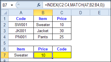
To see how INDEX and MATCH work together, we’ll start with an example that has only 1 criterion. Our price list has item names in column B, and we want to get the matching price from column C.
In the screen shot below, cell A7 has the name of the item that we need a price for – Sweater.
We can enter an INDEX and MATCH formula in cell C7, to get the price for that item:
=INDEX($C$2:$C$4,MATCH(A7,$B$2:$B$4,0))
How the INDEX and MATCH Formula Works
Here’s how the two functions work together:
- MATCH function gets the location of an item in a list
- INDEX function returns a value from a specific location in a list.
So, in our formula:
- the MATCH function looks for “Sweater” in the range B2:B4.
- The result is 1, because “Sweater” is item number 1, in that range of cells.
- the INDEX function looks in the range C2:C4
- The result is 10, from row 1 in that range
So, by combining INDEX and MATCH, you can find the row with “Sweater” and return the price from that row.
Find a Match for Multiple Criteria
In the first example, there was only one criterion, and the match was based on the Item name – Sweater. However, sometimes life, and Excel workbooks, are more complicated.
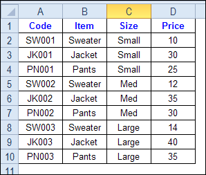
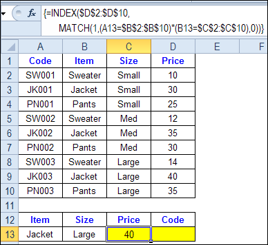
In the screen shot below, each item is listed 3 times in the pricing lookup table. We want to find the price for a large jacket.
To get the right price, you’ll need to use 2 criteria:
- the item name
- the size
Does it MATCH? True or False
Instead of a simple MATCH formula, we’ll use one that checks both the Item and Size columns.
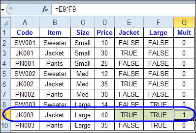
To see how this formula will work, I’ll temporarily add columns to check the item and Size of each item — is the item a Jacket, and is the Size a Large?
Enter this formula in E2, and copy down to E10: =C2=$C$13
Enter this formula in F2, and copy down to F10: =D2=$D$13
- If the Item in column B is a Jacket, the result in column E is TRUE. If not, the result is FALSE
- If the Size in column C is Large, the result in column F is TRUE. If not, the result is FALSE
To see if both results are TRUE in each row, enter this formula in G2, and copy down to G10: =F2*G2
When you multiply the TRUE/FALSE values,
- If either value is FALSE (0), the result is zero
- If both values are TRUE, the result is 1
Only the 8th row in our list of items has a 1, because both values are TRUE in that row.
We can tell the MATCH function to look for a 1, and that will return the information that we need.
Use MATCH With Multiple Criteria
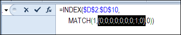
Instead of adding extra columns to the worksheet, we can use an array-entered INDEX and MATCH formula to do all the work.
Here is the formula that we’ll use to get the correct price, and the explanation is below:
=INDEX($D$2:$D$10,
MATCH(1,(A13=$B$2:$B$10) * (B13=$C$2:$C$10),0))
NOTE: This is an array-entered formula, so press Ctrl + Shift + Enter, instead of just pressing the Enter key.
How the Formula Works
In this INDEX and MATCH example,
- prices are in cells D2:D10, so that is the range that the INDEX function will use
- the item name is in cell A13
- the size is in cell B13.
The formula checks for the selected items in $B$2:$B$10, and sizes in $C$2:$C$10. The results are multiplied.
- (A13=$B$2:$B$10)*(B13=$C$2:$C$10)
The MATCH function looks for the 1 in the array of results.
- MATCH(1,(A13=$B$2:$B$10)*(B13=$C$2:$C$10),0)
If you select that part of the formula and press the F9 key, you can see the calculated results. In the screen shot below there are 9 results, and all are zero, except the 8th result, which is 1.
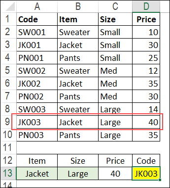
So, the INDEX function returns the price – 40 – from the 8th data row in column D (cell D9).
Get the Product Code
To find the product code for the selected item and size, you would change the formula to look in cells A2:A10, instead of the price column.
Put this formula in cell D13, and remember, this is an array-entered formula, so press Ctrl + Shift + Enter.
=INDEX($A$2:$A$10,
MATCH(1,(A13=$B$2:$B$10) * (B13=$C$2:$C$10),0))
In this example, the product code would be JK003, from cell A9.
Get the Workbook
To get the sample file with the Lookup Multiple Criteria examples, go to the Excel Lookup Multiple Criteria page on my Contextures site.
For more INDEX and MATCH tips and examples, visit the INDEX function and MATCH function page on the Contextures website. This is Example 4 in the sample file section of that page.
_____________
i have 3 column like A, B, C and now i want to formula for A-B=C but in this formula if data is available then by calculation is working fine. but if in some case B Column data is blank then what formula i have to use.
Please help!!!!!
This is a great how and why. I am however getting a #value error because I’m using text, but I’m not sure how to fix that situation as the compare should be returning a number value. essentially I havethe following: index(column A, match(1(column b)*(column c),0)). all columns are text. If I understood correctly I was returning a 1=true,0=false value so I don’t understand the #value error I’m getting. any guidance is appreciated.
I have use this formula to look up value from form but in cell show error #Value!
=INDEX(Timein,)*MATCH(1,(A7=IDList)*(A11=Date),0)
Pleas help me in this problem
Suuuuuuuuper helpful post, Debra, thanks so much!! Very nicely displayed and very clear. Keep up the good work!
Thank you for this tutorial. It has been very helpful.
I do note one problem with it. I’m usually working with data in a variable set of rows or rows that might have blank cells between them. As such, this formula seems to be failing for me.
Using your example, I tried something similar to:
=INDEX($D:$D,MATCH(1,(A13=$B:$B)*(B13=$C:$C),0))but the result was #NUM. I then tried:
=INDEX($D:$D,MATCH(1,(A13=$B$2:$B$11)*(B13=$C$2:$C$11),0))and the return value was 30, the value in the cell just above the desired result. EDIT: I see the mistake in the second code, I forgot to put $D$2:$D$11. It actually does work when I fix that. However, it is curious to me that I may be hitting an Excel array limitation when trying to use full column matching.
A13 and B13 in my example is where I put my values for Sweater and Large.
When I went back to the attempt on my spreadsheet, which was 6201 rows of data, attempted to do the F9 trick on my inner match function, I got a “Formula is too long.” popup error from Excel.
OK, final reply. I figured out what my problem was. There is no array limitation that I was running into. I was confusing a mathematical formula with a string manipulation formula. Still, the $A:$A thing wasn’t working with the example. Now, onto my problem for which there will have to be different solution. (I’ll probably use VBA in a macro.)
When I was first using Match, it was using the first value as my search term. That is, I had a column of data with [nameOfGroup: groupID] and my reference value was only the groupID. So, my Match function looked like (where column A held my indeterminant number of rows of data to be searched and H2 held the groupID being searched):
match("*"&H2,$A$2:$A$6202,0)I modified it, using the example above, to be:
match(1,("*"&H2=$A$2:$A$6202),0)But that doesn’t work (obviously), because I’ve made the new formula a conditional. And the conditional doesn’t work the way I intended it.
Ahh…. now to go stretch my coding brain again.
sorry, final, final post.
My solution, a bit klunky, but it works. Essentially, I use FIND. (SEARCH works, too).
=INDEX($D$2:$D$6202,MATCH(1,FIND(H3,$A$2:$A$6202)/FIND(H3,$A$2:$A$6202))*(I3=$B$2:$B$6202),0))
What is happening is I use the FIND to return the number the value is found within the search term and then divide it by itself, which gives me a 1.
Astute readers will see the problem: “What happens if a match isn’t found?” It will return a divide by 0 error (0/0). Excel handles this situation by putting a #N/A on the line. It shouldn’t matter. You will get the result you want and be able to handle the results not found situations.
I call your page as “EXCEL HEAVEN”
Thanks for the learning! Keep Sharing! 😀