

Use INDEX and MATCH together, for a powerful lookup formula. It’s similar to a VLOOKUP formula, but more flexible — the item that you’re looking for doesn’t have to be in the first column at the left. Watch the video to see how it works (there are written instructions too), and download the sample workbook to follow along.
Excel Lookup With Two Criteria
Watch this video to see how INDEX and MATCH work together — first with one criterion, and then with multiple criteria. Download the sample workbook to follow along, and the written instructions are below the video.
- 0:00 Introduction
- 0:26 Lookup with One Criterion
- 1:52 Test Each Criterion
- 2:22 Test With a Formula
- 3:26 Multiply the Results
- 4:03 INDEX / MATCH Formula
- 5:20 Check the Formula
- 5:57 Get the Sample File
Get Item Price with INDEX and MATCH
To see how INDEX and MATCH work together, we’ll start with an example that has only 1 criterion. Our price list has item names in column B, and we want to get the matching price from column C.
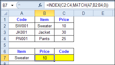
In the screen shot below, cell A7 has the name of the item that we need a price for – Sweater.
We can enter an INDEX and MATCH formula in cell C7, to get the price for that item:
=INDEX($C$2:$C$4,MATCH(A7,$B$2:$B$4,0))
How the INDEX and MATCH Formula Works
Here’s how the two functions work together:
- MATCH function gets the location of an item in a list
- INDEX function returns a value from a specific location in a list.
So, in our formula:
- the MATCH function looks for “Sweater” in the range B2:B4.
- The result is 1, because “Sweater” is item number 1, in that range of cells.
- the INDEX function looks in the range C2:C4
- The result is 10, from row 1 in that range
So, by combining INDEX and MATCH, you can find the row with “Sweater” and return the price from that row.
Find a Match for Multiple Criteria
In the first example, there was only one criterion, and the match was based on the Item name – Sweater. However, sometimes life, and Excel workbooks, are more complicated.
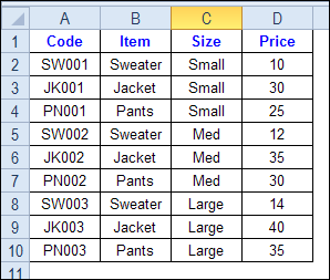
In the screen shot below, each item is listed 3 times in the pricing lookup table. We want to find the price for a large jacket.
To get the right price, you’ll need to use 2 criteria:
- the item name
- the size
Does it MATCH? True or False
Instead of a simple MATCH formula, we’ll use one that checks both the Item and Size columns.
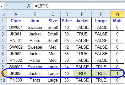
To see how this formula will work, I’ll temporarily add columns to check the item and Size of each item — is the item a Jacket, and is the Size a Large?
Enter this formula in E2, and copy down to E10: =C2=$C$13
Enter this formula in F2, and copy down to F10: =D2=$D$13
- If the Item in column B is a Jacket, the result in column E is TRUE. If not, the result is FALSE
- If the Size in column C is Large, the result in column F is TRUE. If not, the result is FALSE
To see if both results are TRUE in each row, enter this formula in G2, and copy down to G10: =F2*G2
When you multiply the TRUE/FALSE values,
- If either value is FALSE (0), the result is zero
- If both values are TRUE, the result is 1
Only the 8th row in our list of items has a 1, because both values are TRUE in that row.
We can tell the MATCH function to look for a 1, and that will return the information that we need.
Use MATCH With Multiple Criteria
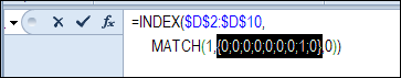
Instead of adding extra columns to the worksheet, we can use an array-entered INDEX and MATCH formula to do all the work.
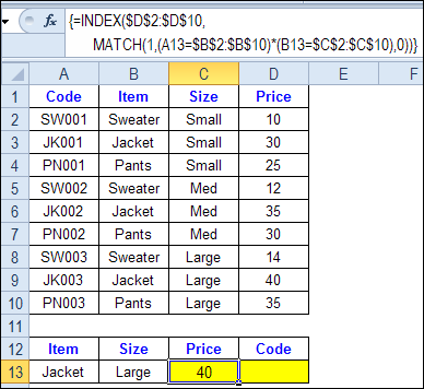
Here is the formula that we’ll use to get the correct price, and the explanation is below:
=INDEX($D$2:$D$10,
MATCH(1,(A13=$B$2:$B$10) * (B13=$C$2:$C$10),0))
NOTE: This is an array-entered formula, so press Ctrl + Shift + Enter, instead of just pressing the Enter key.
How the Formula Works
In this INDEX and MATCH example,
- prices are in cells D2:D10, so that is the range that the INDEX function will use
- the item name is in cell A13
- the size is in cell B13.
The formula checks for the selected items in $B$2:$B$10, and sizes in $C$2:$C$10. The results are multiplied.
- (A13=$B$2:$B$10)*(B13=$C$2:$C$10)
The MATCH function looks for the 1 in the array of results.
- MATCH(1,(A13=$B$2:$B$10)*(B13=$C$2:$C$10),0)
If you select that part of the formula and press the F9 key, you can see the calculated results. In the screen shot below there are 9 results, and all are zero, except the 8th result, which is 1.
So, the INDEX function returns the price – 40 – from the 8th data row in column D (cell D9).
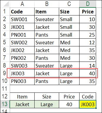
Get the Product Code
To find the product code for the selected item and size, you would change the formula to look in cells A2:A10, instead of the price column.
Put this formula in cell D13, and remember, this is an array-entered formula, so press Ctrl + Shift + Enter.
=INDEX($A$2:$A$10,
MATCH(1,(A13=$B$2:$B$10) * (B13=$C$2:$C$10),0))
In this example, the product code would be JK003, from cell A9.
Get the Workbook
To get the sample file with the Lookup Multiple Criteria examples, go to the Excel Lookup Multiple Criteria page on my Contextures site.
For more INDEX and MATCH tips and examples, visit the INDEX function and MATCH function page on the Contextures website. This is Example 4 in the sample file section of that page.
_____________
I am working with a large amount of data in one worksheet and need to pull data from one field that is within a row that matches three text based criteria into a second worksheet.
I have tried many combinations, but this is my most recent attempt.
=INDEX(‘Zone 11’!$H:$H,MATCH($k11,IF(DataDump!$E:$E=$A11)*(DataDump!$G:$G=”Q1-2015″)*(DataDump!$N:$N=”2015″),0))
Can you help me sort this out?
Hi All ,
i have 3 column; findin lil difficult , can any1 help me 1st match is row ref and 2 nd match is column ref =INDEX(B3:$AJ$50,MATCH($B$1,$F$3:$F$50,0),MATCH($A$1,$F$2:$AJ$2,0))
Is there a way of checking 2 columns to see if they are both a match, and then if they do match, check along that row and look up all of the columns that have an “X” in them and reurn all of the column numbers into a single cell?
EG.
The table I want to look up the culum numbers from looks like:
EXP | TEST | – | 1 | 2 | 3 | 4 | 5 |…| 25 |
2 | 7 | – | X | X | X | X | X |…| X |
11 | 13 | – | | | X | | | | |
13 | 4 | – | | | | | X | | |
13 | 9 | – | X | | X | | | | |
. | . | – | | | | | | | |
. | . | – | | | | | | | |
. | . | – | | | | | | | |
Then in a seperate worksheet, I have the EXP & Test numbers like so:
EXP | TEST | Column No |
52 | 4 | – |
84 | 7 | – |
84 | 12 | – |
. | . | – |
. | . | – |
. | . | – |
. | . | – |
I am wanting to use the values from this 2nd table to look up matching cells in the 1st table (ie when both the EXP AND Test number match) and then look across that column and whenever there is an “X”, it gives back the number of the column and puts it in a single cell in the “Column No.” column.
EG.
EXP | TEST | Column No |
13 | 9 | 1, 3 |
52 | 4 | … |
84 | 7 | … |
Thanks,
Bob
I’m looking for some solution where INDEX MAtch find the output of my keyword based on a condition.
I’m having list of city names with change values in front for each city. In my second sheet i’m calling the value to give me value for City XYZ if the district is ABC.
Currently I’m using ” =INDEX(Sheet1!$D$3:$D$13,MATCH(C3,Sheet1!$C$3:$C$13))”
But the problem is that it pick first come city value.
For Exacmple: In my BASE sheet I’ve Jordan three times under different Districts and each times its value is changed. When i call it from my data entry sheet it picks up the first value and do it again whenever the word “Jordan” comes whereas the value is change for another “JORDAN”
Thanks in Advance,
I got the solution from Sample file Example 4 by customizing 🙂
@Naveed, great! Thanks for letting me know that you were able to get it working.
This formula works great! Thanks so much for posting.
I am not excel savvy, however, was able to follow the instructions and get the formula to work.
Is there a way to combine exact match(case sensitive) to the 2 criteria?
I have a formula {=INDEX(Sheet2!$A1:$H5,MATCH(B2,Sheet2!$A1:$A49),MATCH(D4&A5,Sheet2!$A1:$Z1&Sheet2!$A2:$Z2,0))}. I am looking up for three conditions–if there is a specific string in row 1 and another specific string in row 2 as well as a specific string (a first name) in column A.
I have 3 mock first names and I enter one into a particular cell, and the Index function does it’s thing. I can then enter a different name into that cell and different values will be pulled via INDEX, and so forth. The issue is this formula works for 2 of them, but not the third. They are all formatted as strings (or numbers), and the formula is entered as an array. I am completely baffled. HELP!!!